Imatest Rescharts slanted-edge modules perform highly automated measurements of several key image quality factors using specially-designed test charts. The user never has to manually select Regions of Interest (ROIs).
This page covers results that are (mostly) not derived from the slanted-edges themselves, including
- Noise (best in eSFR ISO)
- Distortion (differing detail in different modules; best with SFRplus and eSFR ISO. Described in detail here.
- Tonal response* (no noise statistics for SFRplus)
- Color accuracy* when used with an SFRplus, eSFR ISO, or SFRreg center charts that contain a color pattern
- Vanishing resolution, aliasing, and Moiré from Wedge patterns in eSFR ISO
- ISO sensitivity* (Saturation-based and Standard Output Sensitivity) for charts with a grayscale pattern, when incident lux is entered
- Image, Geometry, Distortion, Field of View for all charts
*only for charts with tone and/or color patterns. Not in SFRreg (without center chart) or Checkerboard.
Edge-derived sharpness measurements and text (JSON and CSV) output files are covered in Rescharts Slanted-Edge modules, Part 3: Edge Results, which applies to all Rescharts slanted-edge modules. Here are earlier individual pages.
Using SFRplus, Part 3, | Using eSFR ISO, Part 3 | Using SFRreg, Part 3 | Using Checkerboard, Part 3
- Sharpness, expressed as Spatial Frequency Response (SFR), also known as the Modulation Transfer Function (MTF),
- Lateral Chromatic Aberration
|
This page combines results for the four Rescharts slanted-edge modules In many cases we will use SFRplus as an example. Other module produce similar results. |
|
New in Imatest 5.1 Chart MTF compensation has been added to compensate for chart limitations. This can double the maximum megapixel capacity of most charts. Imatest 5.0 Nonuniform lighting perpendicular to the edge can be compensated. This improves the estimate of summary metrics such as MTF50. |
Four introductory pages — SFRplus, eSFR ISO, SFRreg, and Checkerboard — describe each module and explain how to obtain and photograph the chart.
Rescharts Instructions Part 2 shows how to run the modules inside Rescharts and save settings for automated runs.
Results
When calculations are complete, results are displayed in the Rescharts window, which allows a number of displays to be selected. The following table shows the figure that displays specific results. Displays are numbered, but the numbers are different for different modules. Results from slanted-edge measurements are in Part 3.
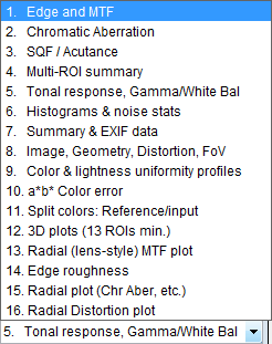 SFRplus display selections
| Slanted-edge Measurement (Part 3) | Display |
| MTF (sharpness) for individual regions | Edge and MTF |
| MTF (sharpness) for entire image | Multi-ROI summary 3D plot Lens-style MTF plot |
| Lateral Chromatic Aberration | Chromatic Aberration |
| Acutance/SQF (Subjective Quality Factor) | Acutance / SQF |
| Edge roughness | Edge roughness |
| Noise (from slanted-edges) | Histograms and noise stats |
| Point Spread Function (approximate) | PSF plot |
| Other measurement (this page) | Display |
| Image, Geometry, Distortion, Field of View | Image & geometry |
| Distortion (geometric– radial plot) | Radial Distortion Plot |
| Tonal response & gamma | Tonal response & gamma |
| Detailed eSFR ISO noise | Detailed noise plot See Color/Tone/eSFR ISO Noise |
| Color accuracy | a*b* Color error Split colors |
| ISO Sensitivity | Tonal response & gamma |
| Uniformity/Light falloff profiles | Color & lightness uniformity profiles |
| EXIF data | Summary & EXIF data |
| Wedge resolution, aliasing, & MTF [eSFR ISO-only] | Wedge aliasing & MTF Multi-wedge plot |
Settings that affect each display will be shown. Most of these settings are not listed in Part 2. They are saved for Auto runs.
Tonal response and gamma display
eSFR ISO and SFRreg center chart
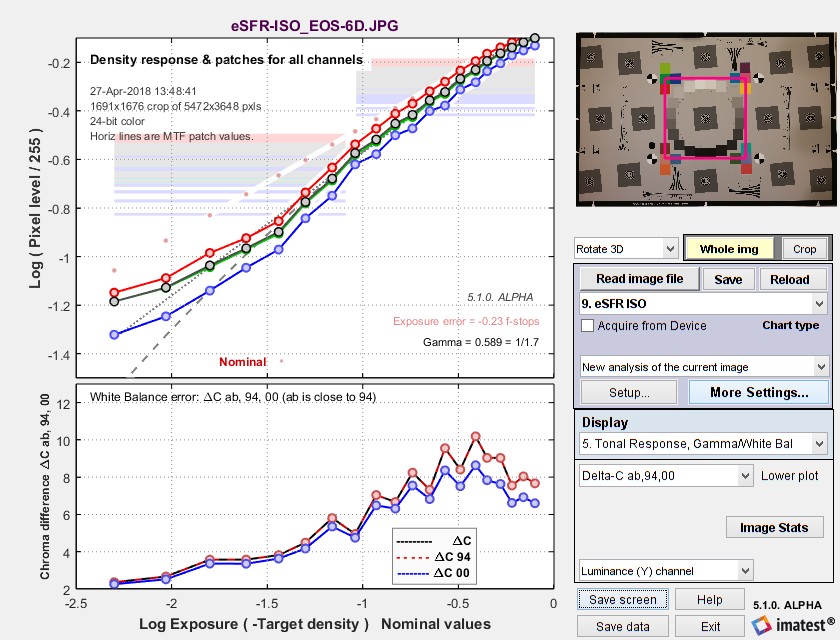 Results in Rescharts window: Tonal response, Gamma, White balance
from the circular grayscale pattern in eSFR ISO or the SFRreg center chart
For SFRplus this display is derived from the 4x5 stepchart pattern, located just below the center of the chart. It resembles the third figure in Stepchart. The upper plot shows the tonal response (also called OECF for Opto-Electronic Conversion Function) for all colors. The lower plot shows the white balance error (deviation from neutral gray) in the three ΔC units shown in the legend. The value of gamma may differ slightly from the values in the Edge response and MTF display because it's calculated differently-- based on the average slope of the light to middle tone squares of the stepchart. The levels of the light and dark portions of the patches used to calculate MTF are shown as pale horizontal lines and as points on the extreme left and right of the upper plot. You can use these lines to see if the patches are within the (relatively) linear region of tonal response (they are in the example on the right). A warning message (Warning: MTF patches may saturate) is displayed if any of the patches are close to saturation (log(pixel level/255) > -0.01; roughly, pixel level > 249 of 255).
Nominal chart densities
| eSFR ISO or SFRreg center chart (20-patch) |
Values from the ISO 14524 Table A.3, 160:1 chart. |
| SFRplus | Linear density steps: 0.05 to 1.95 in steps of 0.10 (different from eSFR ISO) Patch order is shown in Grayscale charts. |
Note that the maximum actual printed density in matte charts is approximately 1.7. Some matte charts are supplied with attached semigloss stickers to increase the maximum density.
Plot settings area
This area (lower-right of the Rescharts window, below Display) lets you choose which results to display. the contents of this section are different for each plot. Many of the selections are saved for Auto mode plots. The tonal response has only two settings: Channel (described in part 2) and Lower plot, which can one of the following.
| Local Contrast | the derivative of the density response: the local value of gamma |
| Delta-C ab, 94, 00 | The indicated color difference (omitting luminance difference) |
| Delta-T | The deviation of the correlated color temperature (degrees Kelvin) from neutral |
| Mireds | micro-inverse degrees: a measure of color error used for calculating correction filters. |
opens the current image in the Image Statistics module, which allows portions of the image to be examined in detail. It provides cross-sections, historgrams, Fourier transforms, and more.
Color & lightness uniformity profiles
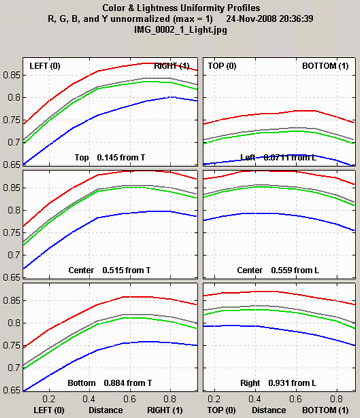
Uniformity profiles
SFRplus and Checkerboard
This display is similar in some respects to the profile plots in Light Falloff. It consists of profiles of the light areas (average values of rectangles between squares). Left-to-right profiles of the top, middle, and bottom of the image are shown on the left side of the display, and top-to-bottom profiles at the left, center, and right of the image are shown on the right. The following display options are available.
R, G, B, and Y unnormalized (max = 1)
R, G, B, and Y normalized (max = 1)
R, G, B, and Y unnormalized (max = 255)
R/G (Red) and B/G (Blue) unnormalized
R/G (Red) and B/G (Blue) normalized (max = 1)
Delta-L* (gray), a* (R), b* (B), chroma c* (G)
For best results with this display, you should make every effort to illuminate the target uniformly using techniques in The Imatest Test Lab. Brightness-related results (R, G, B, Y, and Delta-L*) cannot be measured as accurately as with Light Falloff, where the recommended technique calls for a clear uniform image field photographed through opal diffusing glass. But they can still be useful. The color ratios (R/G, etc.) can be especially useful for diagnosing uneven color response.
Image, Geometry, Distortion, FoV
All modules
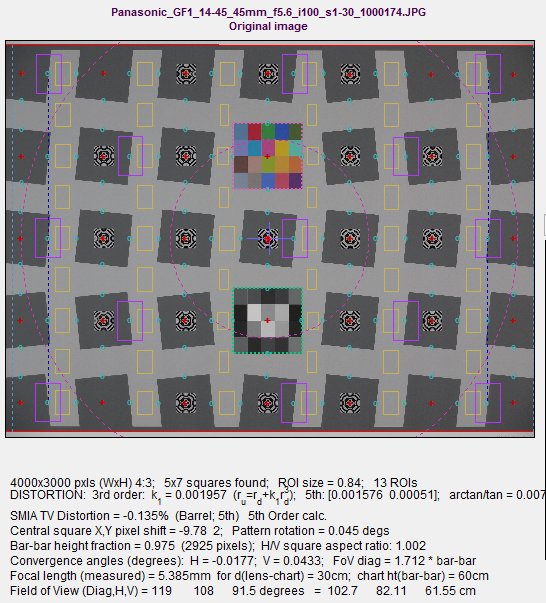 Image, Geometry, Distortion, FoV display
This display allows several aspects of the image to be viewed in detail. It shows the selected regions for MTF/noise analysis (violet rectangles), the yellow rectangles used for generating the uniformity profiles in SFRplus, and the red horizontal curves used to measure distortion in SFRplus). Display options include
| Original Image | Extreme Lighten (HSL) |
| Rec channel | Lighten (HSV) |
| Green channel | Lighten 1 bit |
| Blue channel | Lighten 2 bits |
| Color: Boost Sat. 4X | Original w/5x5 grid |
| Color: Boost Sat, 10X | Original w/5x7 grid |
| Lighten (HSL) | Original w/11x15 grid |
A number of geometrical results are shown beneath the image.
Distortion statistics are described in detail in SFRplus Distortion and Field of View Measurements. You can view the distortion-corrected image using a checkbox in the Display area on the lower-right of the Rescharts window.
- WxH of image in pixels; m x n squares found; ROI size (referencing input setting), number of ROIs for MTF, etc. (not for profiles).
- SMIA TV distortion is the simplest overall measure of distortion. it is positive for pincushion distortion and negative for barrel distortion.
- Third order distortion coefficient k1. ru = rd + k1 rd3 = where ru is the undistorted radius and rd is the distorted radius. r is normalized to the center-to-corner distance. k1 > 0 for barrel distortion and k1 < 0 for pincushion.
- Fifth order distortion coefficients h1 and h2 . ru = rd + h1 rd3 + h2 rd5 A relatively large value of h2 with a different sign from h1 may indicate "wave" or "moustache" distortion, where the predominant distortion goes from barrel to pincushion (or vice-versa) as radius increases.
- Arctangent/tangent distortion coefficients are also calculated and included in the CSV output file.
- Field of View (FoV) is calculated from the selected distortion calculation or the best of three calculations (3rd,order, 5th order, arctan/tan, i.e., the calculation with the least optimizer error).
- x,y coordinates of the center of the middle square relative to the image center.
- The average rotation of the pattern in degrees (>0 for clockwise)
- The bar-to-bar vertical height as a fraction of the image height and in pixels.
- Convergence angles (degrees). These are the result of perspective distortion, when the camera is not pointed directly at the target or is misaligned. The horizontal convergence angle (related to yaw) is shown below: calculated by extrapolating the horizontal bars to the top and bottom. A positive angle has a vortex to the left. In the illustration below the pairs of solid red lines at the top and bottom are parallel (to fit the image on the page).
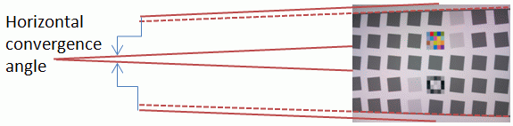
Perfect alignment would be x,y coordinates, rotation, and H,V convergence = 0. Marks may be added to the top and bottom white space of the SFRplus image to facilitate alignment. Vertical convergence angle is derived from lines connecting the right sides of the left-most squares and the left sides of the right-most squares (shown as vertical blue dashed lines - - - above). With fisheye (strongly barrel-distorted) lenses the chart must be precisely centered for the convergence angle measurement to be meaningful.
- measured focal length of the lens is displayed when Bar-to-bar chart height in cm, Lens-to-chart distance in cm, and Pixel spacing (pitch) have been been entered. It is written to the CSV output file if calculated. Equations: Magnification M is bar-to-bar height (on the sensor) / bar-to-bar height (on the chart). For Lens-to-chart distance f1, lens-to-sensor distance f2 = f1M. Using the thin lens equation, focal length f = 1/(1/ f1+1/ f2).
- Field of view calculations include the effects of distortion (the best of 3 models is used). FoV in centimeters (cm) is displayed if the bar-to-bar vertical distance (in the chart center for pre-distorted charts) is entered. FoV in degrees is displayed if the lens-to-chart distance in cm is also entered.
A particularly interesting display is available when you click Crop to ROI (or Crop to 1/2 ROI). The ROI is displayed large enough so its blur is clearly visible and can be compared with Edge and MTF plots and summary results.
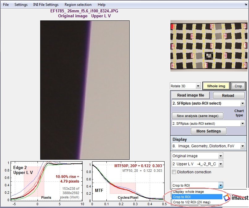 Image, Geometry, Distortion, FoV display, showing Crop to ROI, which allows
the edge appearance (enlarged) to be compared to Edge and MTF results.
Example: highly distorted Checkerboard image with lines and arrows
The relationship between the original and corrected image can be displayed (in Checkerboard-only) when Display arrows & lines is selected in the Display options area of the More settings window. The lines in the original image (below, left) give a good visual indication of how well the calculated coefficients correct the distortion.
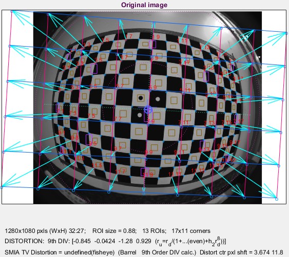 Original image Original image | 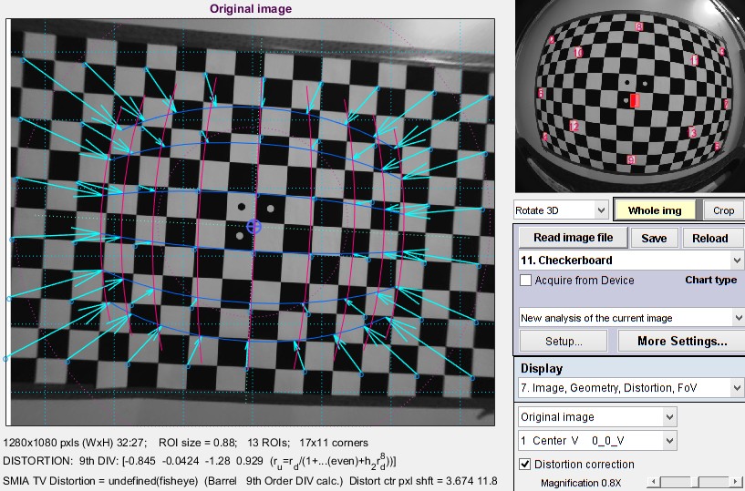 Corrected image Corrected image |
The magnification for the corrected image can be adjusted a slider on the lower-left of the Rescharts display area.
Radial distortion plot
The radial distortion plot adds considerable detail to results in the Image, Geometry, Distortion, FoV display. This plot has four display options: 1. Delta-r, or 2. Lens Geometric Distortion (LGD), 3. r undistorted (ru), or d(LGD)/d(ru). LGD is shown below.
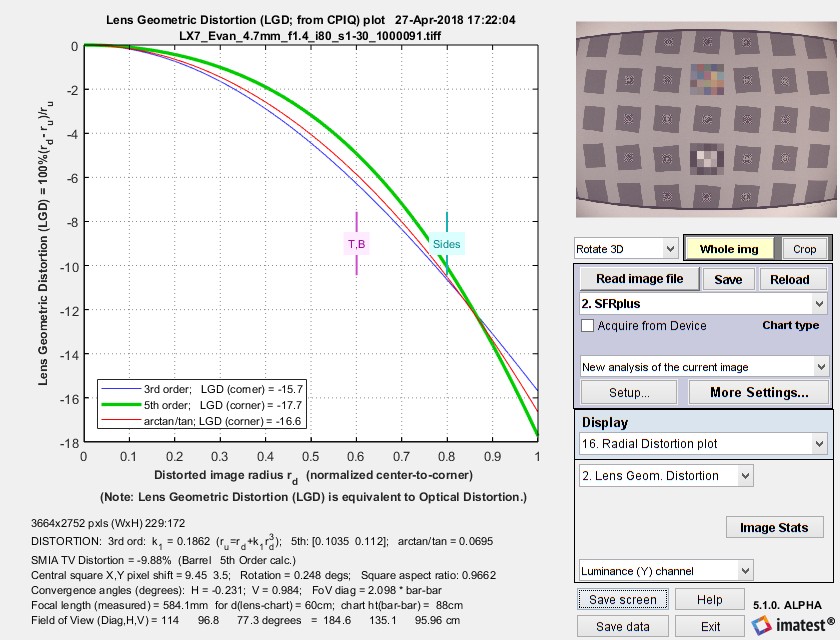 SFRplus Radial Distortion plot showing Lens Geometric Distortion 100% ( rd – ru)/ru
The plot contains
- the change in radius Δr (normalized to the center-to-corner distance, i.e., the half-diagonal) as a function of the distorted (input) radius rd.
Δr = r(undistorted) – r(distorted) = rd – ru - Lens Geometric Distortion (LGD), which is included in the CPIQ Phase 2 specification, and is equivalent to Optical Distortion (defined by Edmund Optics).
LGD = 100% ( rd – ru)/ru - Undistorted radius, ru
- Curvature d(LGD)/d(ru). This curvature (new in Imatest 5.0) may be useful for determining the visual degradation caused by distortion, which is likely to be proportional to the maximum-minimum values. A change in sign may be a better indicator of mustache (wave) distortion than a change in 5th order polynomial sign (which isn’t always calculated).
The solid lines show results for correction formulas: ru = rd + k1 rd3 (3rd order; blue); ru = rd + h1 rd3 + h2 rd5 (5th order; green); or the arctan/tan equations (red). The best fit (5th order in this case) is shown in bold. With these equations |Δr| often increases as a function of r(distorted), i.e., it tends to be largest near the image corners. The selected value (or the one with the least error, err) is shown in boldface.
The radial plot is used to compare results from several Imatest distortion modules in Distortion: Methods and Modules.
Summary & EXIF dataAll modules This plot contains summary results for individual ROIs and EXIF data (metadata that describes camera and lens settings). When first installed, Imatest reads EXIF data from JPEG files only. Enhanced EXIF support requires a special download of ExifTool, described here.EXIF data may be viewed at any time from any display by clicking File, View All EXIF Data. | 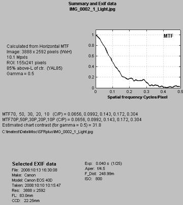 Summary & EXIF data |
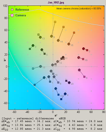
Color analysisSFRplus, eSFR ISO, and SFRreg center chart A color analysis is available for images that contain the optional SFRplus color pattern, which consists of 20 colors in 4 rows and 5 columns. 18 of the 20 colors are close to the colors of the industry-standard 24-patch color chart. The other two are on the yellow and blue sides of neutral gray. To obtain a color analysis,
Two displays are available in the color analysis. The a*b* color error display, shown on the right, is similar to displays in Colorcheck and Color/Tone Interactive. This display shows the reference (nominal) {a*,b*}values as squares and the camera (measured) values as circles. Normally the mean and maximum values of ΔE*ab, ΔC*ab, ΔE*94, ΔC*94, ΔE*00 and ΔC*00 are displayed.
SFRplus chart with optional color pattern The Split (Reference/Input) display is shown on the right. The bottom shows statistics for Row 2, Column 4, obtained by clicking in the Display area on the lower right (not shown). To turn off the probe, click outside the image (in the current version, you need to ckickon the text below the image. This should be fixed in a future version.) When the Probe is off the mean and maximum values of ΔE*ab, ΔC*ab, ΔE*94, ΔC*94, ΔE*00 and ΔC*00 are displayed. |
 a*b* color error a*b* color error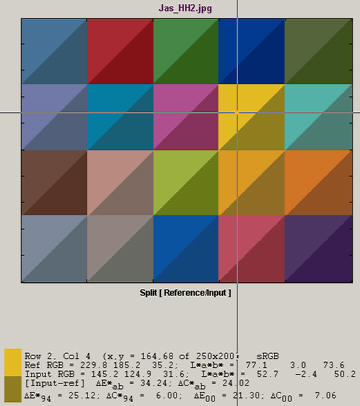 Split view, showing Probe results Split view, showing Probe results |
Noise ploteSFR ISO and SFRreg center chart eSFR ISO can display several types of noise, measured from the grayscale patches surrounding the center of the chart, including all types of noise calculated by Color/Tone Interactive and Color/Tone Auto (standard pixel noise, chroma noise, scene-referenced noise, sensor (raw) noise, and ISO-15739 visual noise). SNR (Signal-to-Noise Ratio) can also be displayed as a ratio or in dB. Instructions for selecting the noise display and x-axis and descriptions of the noise displays are on Color/Tone and eSFR ISO Noise. The figure on the right— simple pixel noise, expressed as a percentage of the maximum pixel value— is one of the simpler noise displays. Noise plot (for simple pixel noise) | 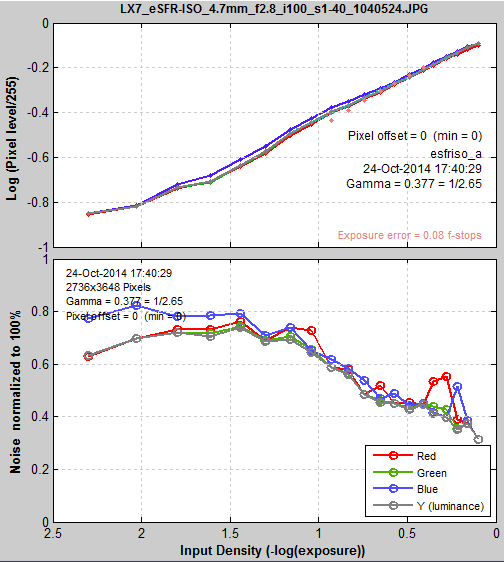 |
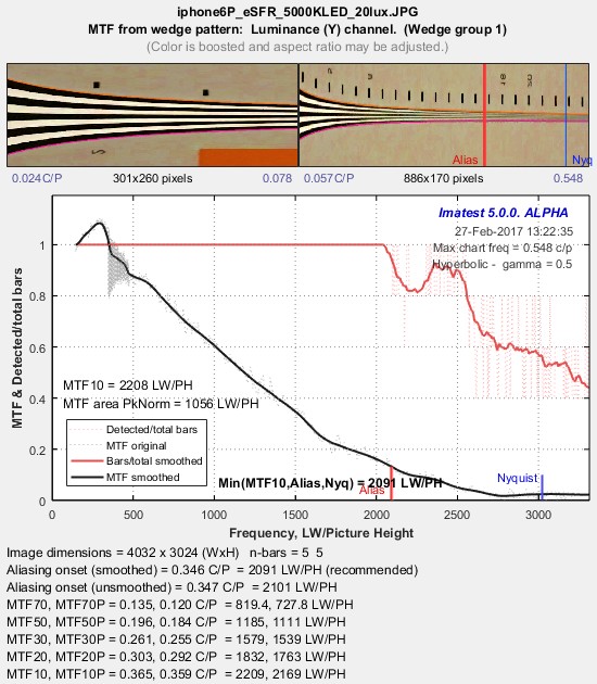
Wedge MTF and Aliasing ploteSFR ISO-only If the Enhanced or Extended chart has been photographed and the Wedge checkbox in the eSFR ISO Setup window has been checked, four or more wedge pairs are automatically detected, and one of two results for each pair (MTF and Aliasing onset, shown on the right, and Moiré) can be displayed. These plots are described in detail in the Wedge module page. Wedge MTF and Aliasing onset plot |
 |
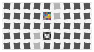
Multi-Wedge plot
eSFR ISO-only
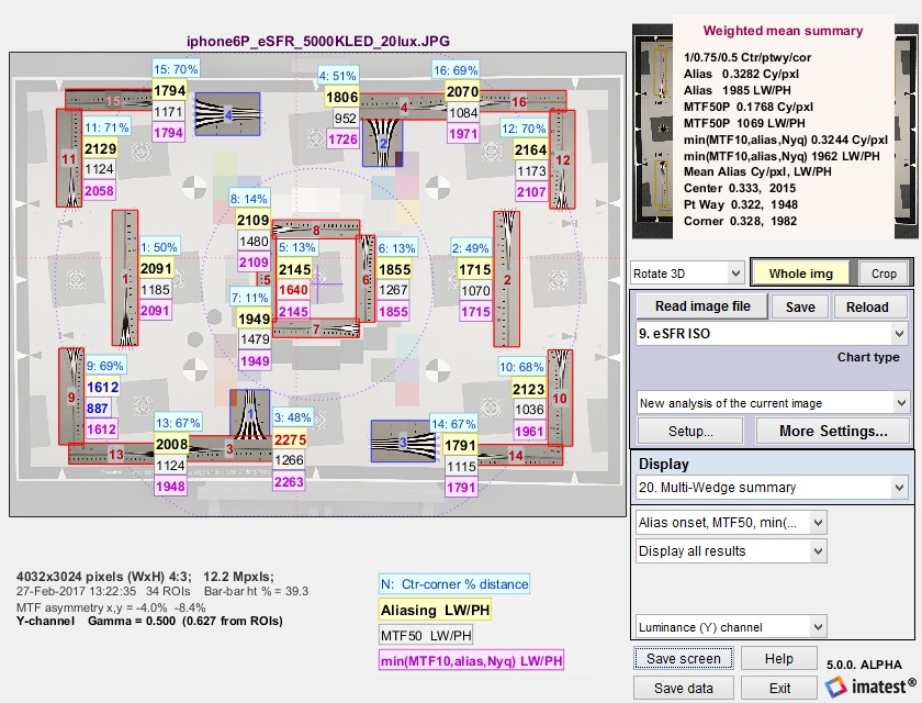
The Multi-Wedge plot shows a summary of results for all wedges. It is the exact counterpart of the Multi-ROI (edge) summary plot for slanted-edges.
|
The multi-ROI (multiple Region of Interest) summary, shown in the Rescharts window (above), contains a summary of eSFR ISO wedge results. The upper left contains the image in muted gray tones, with the selected high frequency wedge regions surrounded by red rectangles and displayed with full contrast. The low frequency wedge regions, which are primarily for low frequency normalization, are inside blue rectangles. Up to four results boxes are displayed next to each region. The results can be selected in the the Display options area on the right, below the Display selection. There is a legend below the image. |
Alias onset, MTF50, MTF20 Results selection |  View selection View selection |
Notes:
- The onset of aliasing is the frequency where the number of detected bars (smoothed to reduce sensitivity to noise) drops to 95% of the low frequency value. It is only indicative of aliasing on relatively sharp systems (good lenses in good focus, so there is some energy around the Nyquist frequency).
-
min(MTF10, alias, Nyq) (the minimum of MTF10, the onset of aliasing, and the Nyquist frequency (0.5C/P)) is the proposed ISO 16505 resolution metric (selected because MTF10 is not robust). See "Measuring MTF with wedges: Pitfalls and best practices" (presented at the Electronic Imaging 2017 conference).
Summary
- SFRplus analyzes images of the SFRplus test chart, ideally framed so that there is white space above and below the horizontal bars in the chart, i.e., so neither bar runs off the top or bottom of the image. The white space should be between 0.5% and 25% of the image height. SFRplus can work without the bars, but distortion and field of view are not calculated. The bars may run off the sides of the image. Interfering patterns (bars, etc.) outside the chart should be kept to a minimum.
- eSFR ISO should be framed to the registration marks are well inside the image. Where possible the entire chart should be inside the image. eSFR ISO has less spatial detail than SFRplus, but has wedges and larger tonal patches that allow much more detailed noise analysis.
- SFRreg is highly flexible, and can include individual charts facing the camera with angular fields of view well over 180 degrees.
- Checkerboard uses a simple checkerboard (chessboard) pattern that works over a wide range of distances: chart framing is not critical.
- Lighting should be even and glare-free. Lighting and alignment recommendations are given in The Imatest test lab.
- The first time any of these modules is run, it should be run through Rescharts. This allows
- parameters to be adjusted and saved for later use in the automatic version, which is opened with a button in the Imatest main window.
- results (listed above) to be examined interactively in the Rescharts window.
- The Auto buttons in the left column of the main Imatest window runs the corresponding module in full automatic mode using settings saved from the most recent Rescharts run. Batches of files can be run.
| Feature | SFRplus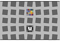 | eSFR ISO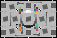 | SFRreg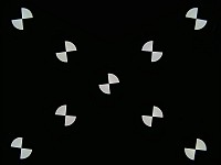 | Checkerboard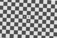 |
| Sharpness map detail | High | Medium | Depends on arrangement | High |
| ISO-standard chart design | – | ♦ | – | – |
| Color analysis | ♦ | ♦ | * | – |
| Tonal response (OECF) | ♦ | ♦ | * | – |
| Noise analysis | Limited | ♦ | * Limited | Limited |
| Distortion | ♦ | Limited | – | ♦ |
| Geometry | ♦ | ♦ | * | ♦ |
| Features and recommended uses | Imatest's original automatically-detected chart, in use since 2009. robust and versatile. Some white space recommended above and below top and bottom bars. More spatial and distortion detail than eSFR ISO. | ISO-standard chart design. Includes wedge analysis. Supports detailed noise analysis. |
Several individual charts are typically placed around the image field. Works with *Available with SFRreg center chart in Imatest 5.0+. FoV is omitted from geometry. | Relatively insensitive to framing: can zoom in or out as long as distance is large enough so chart quality is not an issue and there are detectable corners. |
♦ denotes strong support; – denotes no support.
Links
How to Read MTF Curves by H. H. Nasse of Carl Zeiss. Excellent, thorough introduction. 33 pages long; requires patience. Has a lot of detail on the MTF curves similar to the Lens-style MTF curve in SFRplus. Here is an interesting list of Zeiss technical articles. Their (optical) MTF Tester K8 is of some interest.
Understanding MTF from Luminous Landscape.com has a much shorter introduction.
Understanding image sharpness and MTF A multi-part series by the author of Imatest, mostly written prior to Imatest's founding. Moderately technical.
Bob Atkins has an excellent introduction to MTF and SQF. SQF (subjective quality factor) is a measure of perceived print sharpness that incorporates the contrast sensitivity function (CSF) of the human eye. It will be added to Imatest Master in late October 2006.
How to Measure MTF and other Properties of Lenses by Optikos.