Local Magnification

Introduction

Local magnification is an intuitive metric that can be used to evaluate geometric distortion in images. It maps object magnification (in both radial and tangential directions) with image field height.

Imatest version 26.1 added calculation of local magnification and associated metrics based on the method of Wang et al. [1].

Imatest extends the methods presented in the paper by offering configurable settings, automated processing, and expanded outputs, allowing the method to be applied effectively for a range of camera types and test objectives. As described in the paper, additional metrics can be derived from local magnification data including radial/optical distortion percentage, TV distortion metrics, field of view, and classification of the lens projection method / mapping function. Imatest can perform these additional calculations as part of the analysis. 

Calculation of local magnification is currently available for Checkerboard analysis and must be explicitly enabled in the settings for the target.

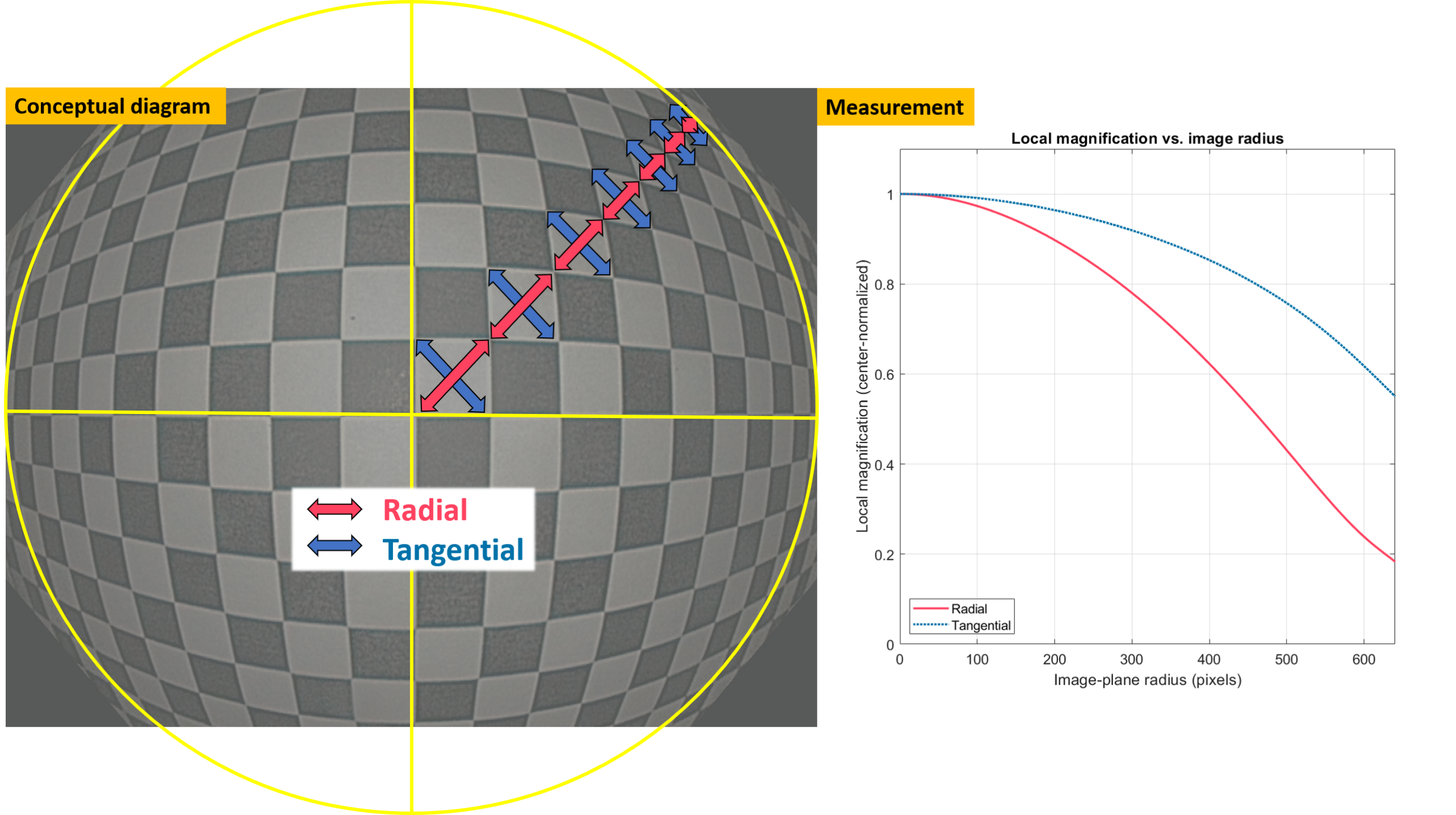
Key Assumptions

Below are some of the key assumptions behind the measurements.

• The geometric distortion is radially symmetric.
• The center of distortion coincides with the numeric image center; however, Imatest provides the option to instead use the centermost detected point as the origin.
• The radial mapping function can be well-modeled by a polynomial. 
• The target grid plane is positioned perpendicular to the optical axis of the camera under test, with one grid point placed at the image center and the central grid row and column parallel to the image frame. See also instructions for Setup & Capture below.

Example Outputs

Available outputs and visualizations for local magnification include:

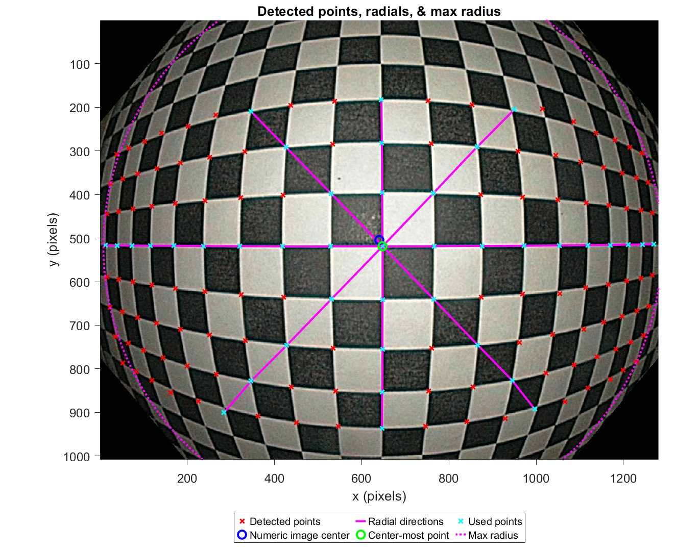
• Detected points, radials, & max radius: A plot showing the image with detected points, radial directions, and the max radius (circle) overlaid. The points along the selected radial directions are used for calculations.
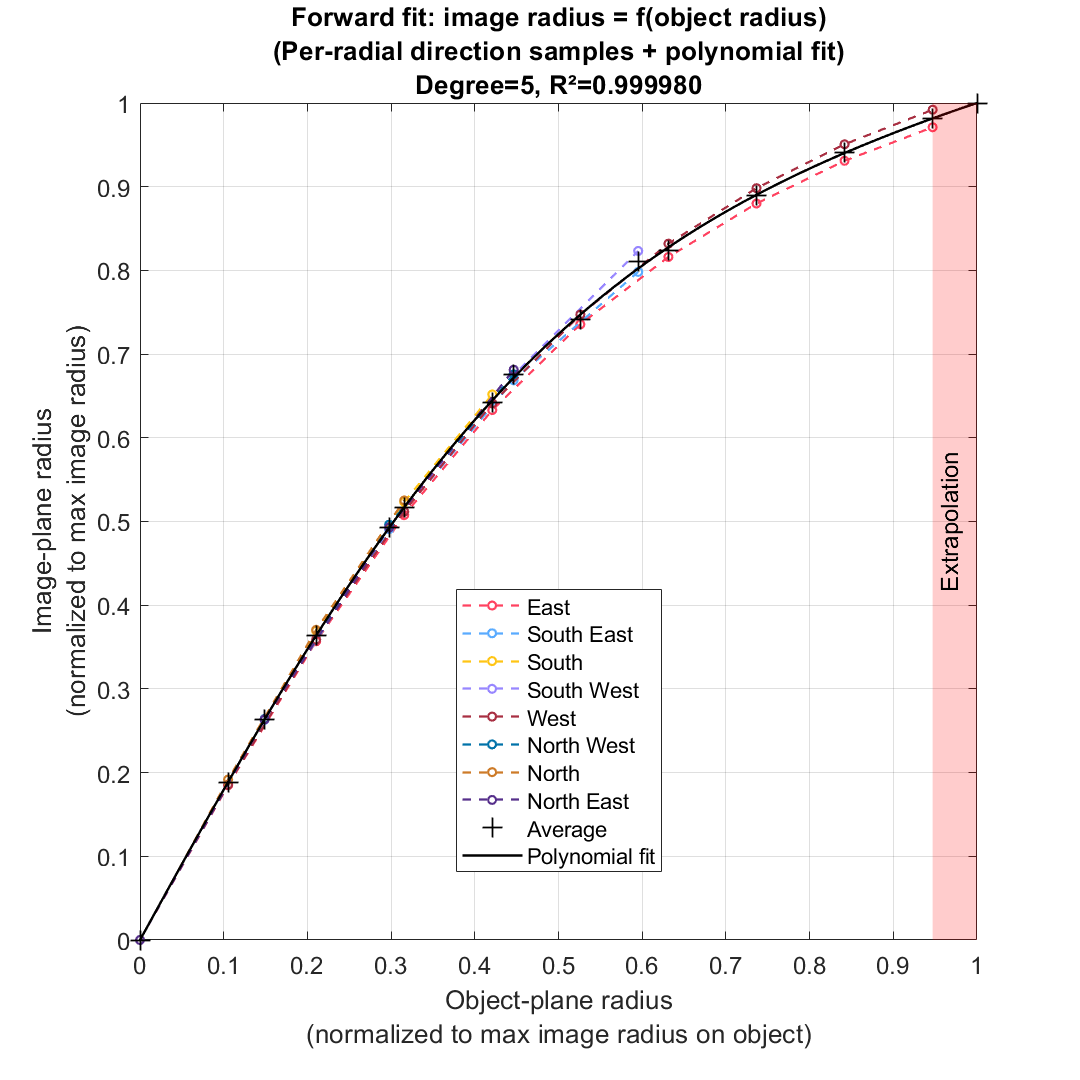
• Image vs. object radius (forward fit): A plot showing image radius vs. object radius, with samples from each radial direction and the polynomial fit for image radius as a function of object radius in the normalized domain. Samples from each direction are averaged by common grid-step distance before computing the polynomial fits.
• Object vs. image radius (inverse fit): A plot showing object radius vs. image radius, with samples from each radial direction and the polynomial fit for object radius as a function of image radius in the normalized domain.
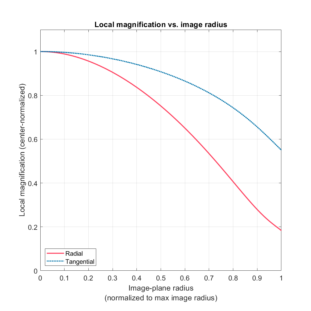
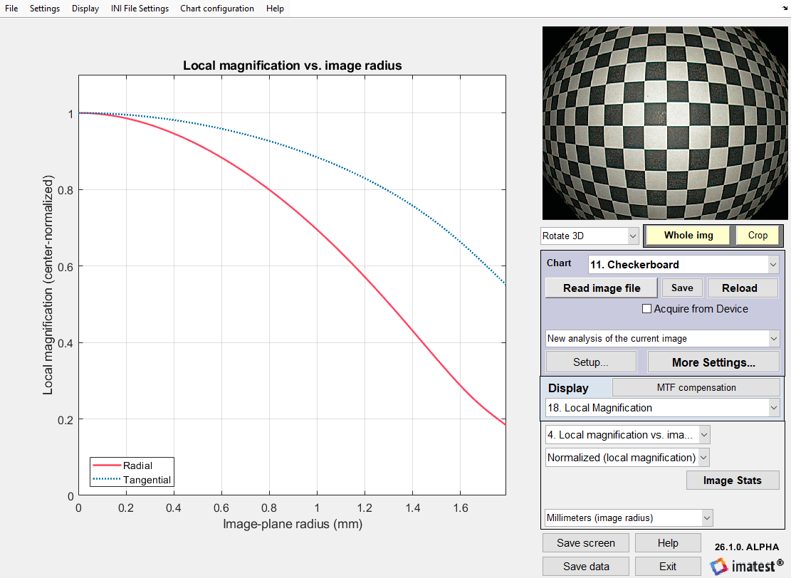
• Local magnification vs. image radius: A plot showing local magnification (radial and tangential) vs. image radius. This is calculated from the (forward) polynomial fit.
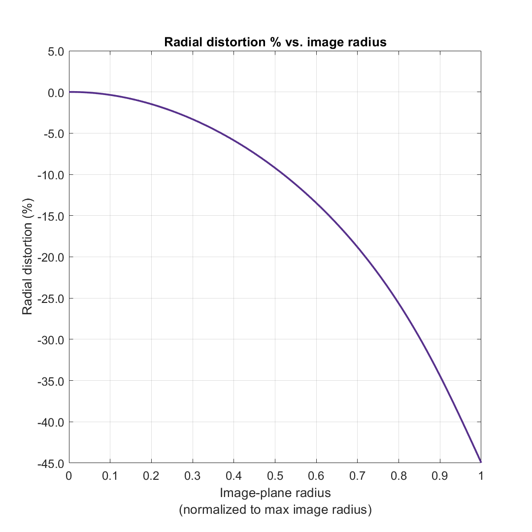
• Radial distortion % vs. image radius: A plot showing radial/optical distortion percentage vs. image radius. This is calculated from the local magnification profile.
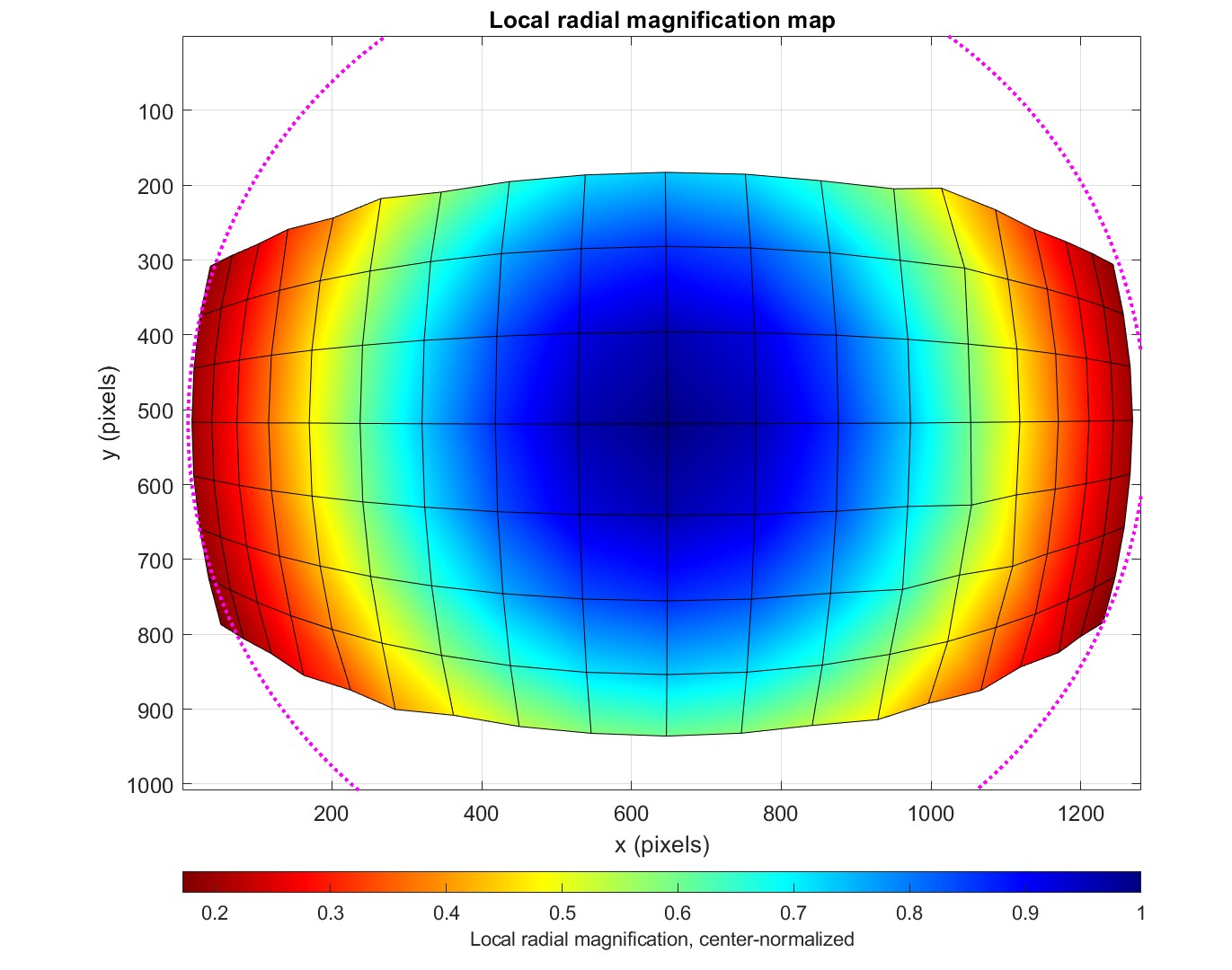
• Local radial and tangential magnification maps: A plot showing the detected grid with local magnification (radial or tangential) evaluated for each point and overlaid as a colormap.
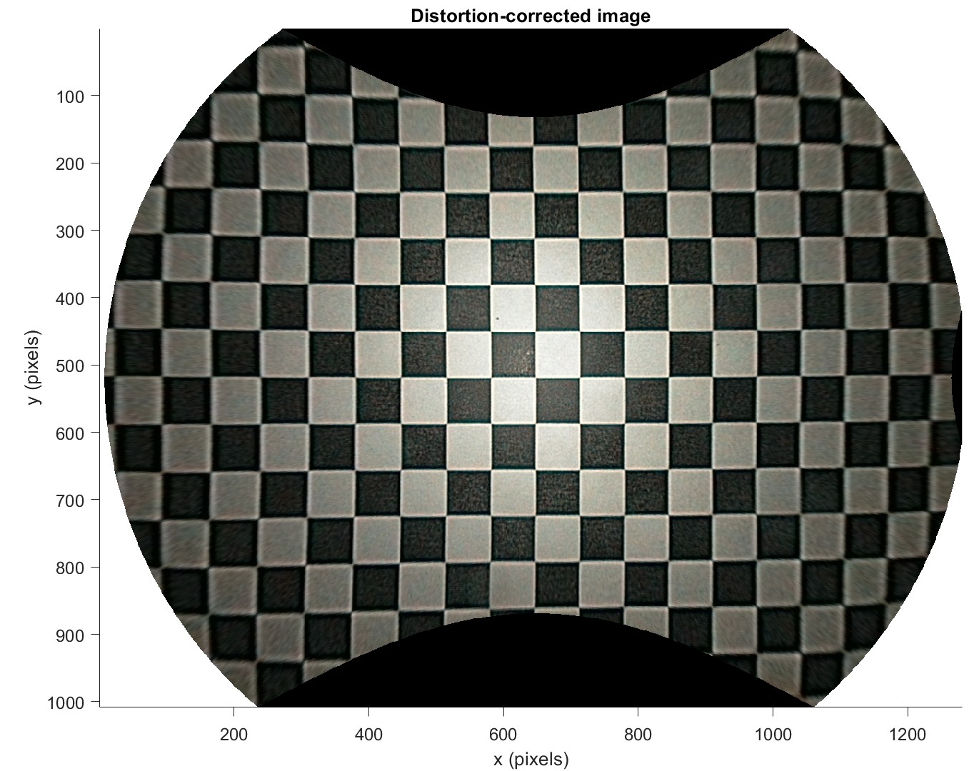
• Distortion-corrected image: A plot showing the distortion-corrected (undistorted) image. The original image is undistorted using the (forward) polynomial fit and resampled to the original image size via linear interpolation.
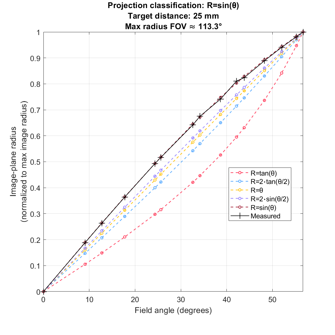
• Projection classification: A plot showing image radius vs. field angle, including canonical projection mapping functions and estimated field of view.

Note: Plot axes units are configurable. Axes for local magnification can be expressed in either absolute terms (image scale factor) or center-normalized. Axes for image radius can be expressed in units of either pixels, millimeters (on image sensor), or normalized (to max image radius). Axes for object radius can be expressed in units of either grid steps, millimeters (on object), or normalized (to max image radius on the object). 

Results and data are also included in Imatest’s standard CSV and JSON output files.

Calculations

Note: Local magnification calculations are separate from other pre-existing geometric distortion calculations in Imatest. Imatest checkerboard analysis produces radial distortion models that are separate from those related to local magnification and are also dependent on separate settings, calculations, etc.

Please see the reference paper for details on the calculations used to measure local magnification and associated metrics. Imatest follows the methods described in the paper with few deviations.

Extensions and deviations from the methods described in paper are noted below.

Extensions

• (Extension) Automatic detection of grid samples (from checkerboard detection).
• (Extension) Configurable multi-directional sampling, allowing use of grid samples along diagonal Radial Directions (NE, SE, SW, NW) in addition to samples from cardinal directions (N, E, S, W).
  • Note: Diagonal Radial Directions introduce samples at additional grid step distances (a diagonal step is ~1.41, while a horizontal or vertical step is 1), providing extra data points for the polynomial fits.
• (Extension) Configurable distortion Origin (center of distortion): numeric image center (from paper) or the centermost point, i.e., the detected grid center (extension).
  • Note: Using the centermost point as the Origin can be useful if the grid center is offset from the numeric image center, as it reduces systematic bias that can destabilize the polynomial fits.
• (Extension) Configurable distortion Max Radius: image sides (left/right or top/bottom, from paper), outermost point (extension), image corners (extension), or custom pixel radius (extension).
• (Extension) Allows use of minimum adjusted R² (instead of standard minimum R²) as criteria for polynomial fit degree searches (via the Use Adjusted R² toggle setting). 
  • Note: Adjusted R² applies a penalty for higher polynomial orders/degrees, which can reduce overfitting.
• (Extension) Produces additional plots/visualizations not found in the paper including:  
  • (Extension) Detected points, radials, & max radius: See example plot above. 
  • (Extension) Local radial and tangential magnification maps: See example plot above. 
• (Extension) Provides relevant data/results in additional units.
  • (Extension) Plot axes units for image radius can alternatively be expressed in units of pixels or millimeters (on the image sensor), in addition to normalized (from paper).
  • (Extension) Plot axes units for object radius can alternatively be expressed in units of grid steps or millimeters (on the object), in addition to normalized (from paper).

Deviations

• (Deviation) The numeric image center is defined as the exact geometric center of the image frame using the IEEE Std 2020 [2] Type IV coordinate system, e.g., [50.5, 50.5] for a 100x100 image. This distinction is primarily semantic.
• (Deviation) A zero intercept is enforced for the forward and inverse polynomial fits that map object radius and image radius in the normalized domain. This constrains the distortion model to pass through the origin, ensuring physical consistency (i.e., a radius of zero in the scene maps to a radius of zero in the image).
  • Note: A zero intercept is not enforced for the initial polynomial fit (object radius in grid steps as a function of image radius in pixels) that is used to estimate the object radius at the selected maximum image radius. Leaving this preliminary step unconstrained can help prioritize fit accuracy at the maximum radius.

Instructions

Instructions for measuring local magnification are below.

Setup & Capture

1. Measure the target’s grid pitch, e.g., the height of a checker.
2. Align the camera with the target.
   1. The target grid plane should be perpendicular to the optical axis of the camera with one grid point (e.g., a checkerboard saddle point) aligned with the numeric image center.
   2. The center row and column of the target grid should be parallel to the edges of the image frame.
   3. The target grid should fill the image frame.
   4. The target grid should have at least one detectable grid point (e.g., a checkerboard saddle point) close to the sides of the image or the desired maximum radius.
3. (Optional – for field of view and projection classification) Measure the distance between the camera entrance pupil and the center of the target.
   1. Note: The camera entrance pupil position is usually somewhere within the camera lens.
4. Capture an image of the target.
   1. The image of the target should be in-focus (sharp) and well-exposed.
   2. The overall quality of the image should be sufficient such that reflections, noise, or other image artifacts do not reduce the accuracy of grid point (e.g., checkerboard saddle point) detection/localization.
   3. (Optional) Multiple images can be captured and then averaged using Imatest to potentially reduce the various effects of noise.

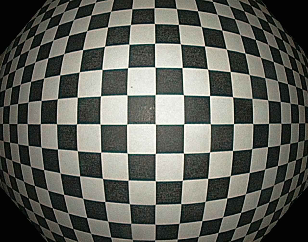
The following example image is from an Olympus EXERA II, which is the same camera device that was tested in the reference paper. According to the paper, the pixel pitch of the image sensor is 2.8 microns. The checker height is assumed to be 4 millimeters and the target distance is assumed to be about 25 millimeters. The camera and target are reasonably well aligned, though not perfectly, as the centermost grid point is slightly offset from the numeric image center.

Imatest Analysis

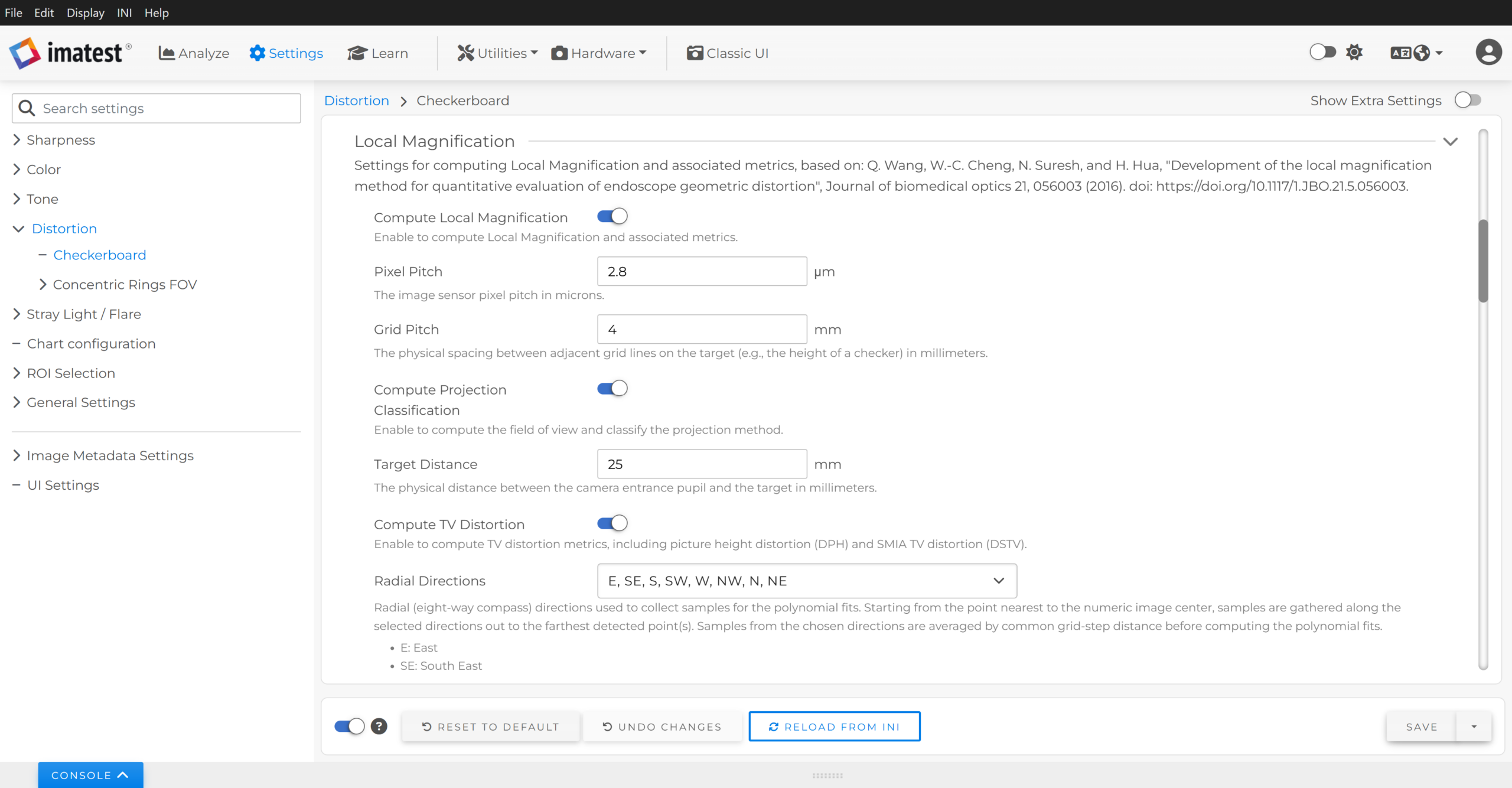
1. In the main window, navigate to Settings > Distortion (or Sharpness) > Checkerboard > Local Magnification.
2. Enable Compute Local Magnification to have Imatest compute local magnification and associated metrics.
3. Enter the image sensor Pixel Pitch in microns.
4. Enter the target’s Grid Pitch, e.g., the height of a checker, in millimeters.
5. (Optionally) Enable Compute Projection Classification to have Imatest compute field of view and classify the lens projection method / mapping function from the local magnification data.
   1. Enter the Target Distance (the distance between the camera entrance pupil and the target center) in millimeters.
6. (Optionally) Enable Compute TV Distortion to have Imatest compute TV distortion metrics from the local magnification data. TV distortion results are included in the JSON/CSV outputs. 
7. (Optionally) Configure remaining calculation settings.
   1. (Optionally) Configure the Radial Directions to choose which points from the detected grid are used for calculations. Samples from the chosen directions are averaged by common grid-step distance before computing the polynomial fits.
   2. (Optionally) Configure the Origin to choose the origin for distortion measurements. 
   3. (Optionally) Configure the Max Radius to choose the image boundary that defines the maximum radius for distortion measurements and normalization.
   4. (Optionally) Configure the Polynomial Fit Degree to choose the degree of the polynomial fits that map image radius and object radius, or to use as the maximum degree for Auto-Select Degree searches.
   5. (Optionally) Enable Auto-Select Degree: Boundary Fit to automatically select the degree for the initial polynomial fit (based on the Minimum R² criteria) used to estimate object radius at the chosen max image radius (Max Radius).
   6. (Optionally) Enable Auto-Select Degree: Normalized Fits to automatically select the degree for the polynomial fit (based on the Minimum R² criteria) used to compute local magnification, as well as the associated inverse fit.
   7. (Optionally) Configure the Minimum R² to specify the lowest acceptable coefficient of determination (R²) a fit must meet for it to be selected during Auto-Select Degree searches.
   8. (Optionally) Enable Use Adjusted R² to have Auto-Select Degree searches evaluated using adjusted R² instead of standard R².
8. (Optionally) Configure the Local Magnification Auto (Batch) Plots settings used for auto/batch analysis. These settings do not affect plots in interactive analysis.
   1. Select which units to use for various plot axes. Selecting multiple units will produce multiple versions of the relevant plots. 
   2. Select the output file format for the plots.
   3. Select which plots to save and/or display.
9. Load and select the image(s) to use for analysis.
10. Select the appropriate target for analysis (i.e., Checkerboard).
11. (Optionally) Configure any target-specific settings such as detection settings, crop, general outputs, etc. by clicking the gear icon on the selected target to open the Setup window.
    1. (Optionally) Configure Checkerboard Auto (batch) settings by clicking Auto Mode settings on the left side of the Setup window. These settings do not affect interactive analysis.
       1. (Optionally) Enable/disable CSV and JSON outputs (both enabled by default).
       2. (Optionally) Change the Folder for saving results (the default behavior creates a subfolder named “Results” in the directory containing the image(s) under test).
12. Run analysis.
    1. Interactive:
       1. From the Setup window, verify that the point detection and coverage is sufficiently good.
          1. (Optionally) Select the NO regions: fast geometry calculation option under ROI selection & analysis to disable non-geometry calculations, such as SFR.
          2. (Optionally) Select Crop borders to choose an image crop which, for local magnification calculations, will only affect checkerboard point detection.
          3. (Optionally) Select Target Detection Settings to configure checkerboard detection settings. Checkerboard detection settings can also be configured from the main window by navigating to Settings > Distortion (or Sharpness) > Checkerboard.
       2. Click OK to continue with analysis.
       3. Wait for analysis to complete.
    2. Auto (batch):
       1. Wait for analysis to complete.
13. View results.
    1. Interactive:
       1. From the Rescharts window, navigate to Display option 18. Local Magnification to see various plots related to local magnification.
       2. Plot axes units are configurable via dropdowns.
       3. Results/data can be saved to standard output files (JSON and CSV) by clicking Save data in the lower-right corner.
       4. A screenshot of the current display can be saved by clicking Save screen in the lower-right corner.
    2. Auto (batch):
       1. Navigate to the output Results folder to find various plot outputs and standard output files (JSON and CSV).
       2. The outputs will reflect the chosen settings under Local Magnification Auto (Batch) Plots, as well as those related to the specific target analysis.

Tips

• Inspect each output.
  • Check the Detected points, radials, & max radius plot.
    • Check that the detected point locations along the chosen Radial Directions (these are the points used for calculations) are sufficiently accurate.
    • Check that the centermost grid point coincides with (or is close to) the numeric image center.
    • Check that there is at least one detected point near the image boundary corresponding to the selected Max Radius.
  • Check the Image vs. object radius (forward fit) plot.
    • The accuracy of the (forward) polynomial fit directly affects the accuracy of local magnification and other derived metrics such as radial distortion percentage. The inverse polynomial fit is utilized exclusively for calculating TV distortion metrics (included in results file outputs). 
    • Check that the samples from each radial direction are not spread apart. Significant spread implies either camera-to-target misalignment, asymmetric distortion, or inaccurate point detection.
    • Check that there are no significant outlier samples that could have biased the averaged samples or the overall measurement, e.g., from inaccurate point detection.
    • Check that the extrapolation (pink) region is small and that the estimated object radius at the selected Max Radius appears accurate.
  • Check the Local magnification vs. image radius plot.
    • One of the benefits of local magnification is that it reflects what one can observe visually.
    • Check that the (center-normalized) local magnification matches what one’s eyes see with respect to how the grid size varies within the image.
  • Check the Distortion-corrected image plot.
    • Check the straightness of the grid in the image. This is a good proxy for evaluating how well the (forward) polynomial fit represents the distortion in the image.
• Understand the limitations of the measurement.
  
  • Radial polynomial distortion models are approximations and may not fully describe the distortion present in the image, especially in the presence of asymmetry or misalignment. 
  • A higher R² for the polynomial fits represents a better fit to the data, but not necessarily a better fit to the actual radial distortion in the image.
    • Use Adjusted R² to penalize higher order models.
    • For stable model outputs, specify the Polynomial Fit Degree and disable Auto-Select Degree searches.
  • Measurements in extrapolated regions are generally less reliable. Any radii beyond the outermost grid point included in the polynomial fits must be extrapolated.
    • To minimize extrapolation, ensure at least one detected grid point lies near the selected Max Radius boundary (e.g., image sides, corners, or custom radius). If points exist at radii beyond the selected Max Radius, the boundary sample is determined via interpolation. If Max Radius is set to the Outermost detected point, the boundary sample is defined directly by measured data, requiring no interpolation or extrapolation.
    • The accuracy of the extrapolated region will directly affect the accuracy in corresponding areas of other outputs, such as local magnification at the edge of the field.
      • For example, the results in the reference paper show local radial magnification taper off and then increase at the edge of the field instead of continuing to decrease (Table 1 and Fig. 11). This region is likely erroneous (we expect the magnification to continue to decrease at the edge of their barrel-distorted image), further supported by their distortion-corrected image (Fig. 15) which exhibits significant curvature at the edges. This error is effectively caused by underestimating the object radius at the max image radius (image sides) via extrapolation. The authors attribute some of this error to inaccurate grid point localization near the image edge (in Section 4.2) which can contribute to such behavior. 
• Review relevant background material.
  • The reference paper provides detailed methodological information and background theory. 
  • The Wikipedia page for "Fisheye Lens" has a decent description of canonical lens projection methods / mapping functions.

Results

See the separate Local Magnification Results page for documentation of the JSON/CSV outputs.

References

- Q. Wang, W.-C. Cheng, N. Suresh, and H. Hua, “Development of the local magnification method for quantitative evaluation of endoscope geometric distortion,” J. Biomed. Opt., vol. 21, no. 5, p. 056003, 2016, doi: 10.1117/1.JBO.21.5.056003. ↩