Measure color accuracy, tonal response, and noise from a large variety of test charts
Imatest 2020.1 We have added support for the TE269V2 and V3 Dynamic Range chart, which have the same layout as our 36-patch DR chart, but a different patch order. Reference files are now available. |
|
Using Color/Tone Interactive (formerly Multicharts) – Interactive analysis of color & grayscale test charts Using Color/Tone Auto – Fixed (batch-capable) analysis of color & grayscale test charts Color/Tone / eSFR ISO Noise – including chroma, sensor (RAW), and visual noise Simatest: Overview – Concise introduction to Simatest: Imatest's Camera/Image Signal Processing (ISP) simulator Image Sensor Noise – measurement and modeling – using raw files for image sensor Dynamic Range and Simatest Dynamic Range – a general introduction with links to Imatest modules that calculate it. Color Correction Matrix (CCM) Calculate a matrix (usually 3×3) for correcting image colors (often from RAW images) |
Introduction
Imatest™ Color/Tone Interactive analyzes images of most popular color and grayscale test charts for color accuracy, tonal response, noise, ISO sensitivity, and Dynamic Range (for transmissive grayscale charts) using a highly interactive user interface. It can be used to measure white balance and color response for a wide range of lighting conditions and scenes. It can also display the tonal response of monochrome charts (or monochrome portions of color charts). A color correction matrix (CCM) can be calculated and used to correct images. The Color/Tone Auto (Multitest) module performs the same analyses using a non-interactive (fixed; batch-capable) interface.
(older, more limited fixed modules).
| Color/Tone (Interactive and Fixed) | Colorcheck | Stepchart | |
|
Description and charts supported | Recent modules that can analyze a large number of popular color and grayscale test charts. Highly versatile. Comes in both interactive and fixed versions. | Older (legacy) module that analyzes the X-Rite 24-patch Colorchecker-only | Older (legacy) module that analyzes most popular grayscale test charts |
| Noise, SNR | A large variety of noise, SNR and Dynamic Range measurements are supported, described in Color/Tone/eSFR ISO noise. | Only simple and scene-referenced noise and SNR are supported. | |
| Color Correction Matrix (CCM) | Can be calculated from most supported color charts. (Charts should contain patches with at least 9 distinct hues and as well as grayscale patches). | no | N/A |
| Dynamic Range (DR) | Imatest Dynamic Range (from transmissive charts), ISO 15739 DR (extrapolated from reflective charts) | no | Imatest DR-only |
| Note: If you are planning to do DR testing, please read the instructions in Dynamic Range. | |||
| Image sensor noise model | The image sensor noise model is the heart of Simatest, the Camera/ISP simulator. Enables camera performance to be simulated for a wide range of conditions. | N/A | no |
The most popular supported test charts are shown in the table below.
A full set of charts and a guide to their use is in
Color/Tone Test Chart Reference & Guide
 Colorchecker |
 IT8.7 IT8.7 |
 Colorchecker SG | ||
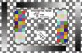 Universal Test Universal TestTarget (UTT) |
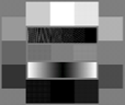 ISO-15739 |
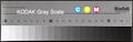 Q-13 (linear grayscale) |
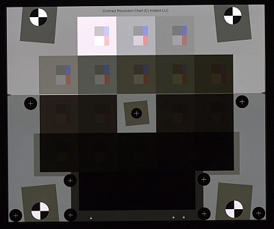 Contrast Resolution Contrast Resolution | |
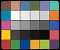 ColorGauge ColorGauge(Micro, Nano, etc.) | 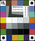 RezChecker RezChecker |
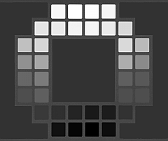 TE269, TE269V2 or TE269, TE269V2 orV3 (3 versions) |
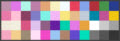 General mxn charts (L*a*b* reference file required) |
 ISO-14524 |
|
Many other charts are supported, including SFRplus and eSFR ISO color patterns
(not automatically detected in Color/Tone), SMPTE/Hale Color Bars (6 patches), and TE226 (9x5) color chart. These charts are described in more detail below; the full set of charts is presented in Color/Tone Test Chart Reference & Guide | ||||
Getting started
Color/Tone Interactive QuickstartPhotograph the chart, using even glare-free lighting. Color and grayscale chart images usually should not fill the frame (1200 vertical pixels is usually sufficient). Filling the frame can cause light falloff issues. Open Color/Tone Interactive. Select the chart type or (if the type is correct) press Read image file. There are some special chart types.
Select the image file to read. Select the region (ROI), following the instructions. You may need to make a coarse region selection followed by a fine selection. Several charts allow automatic region selection. Select the Results Display. Because Color/tone Interactive is highly interactive you can change the Color space, reference file and other settings. You can calculate a Color Correction Matrix (CCM). Many saved settings are shared with Color/Tone Auto (formerly Multitest). |
Photograph or scan the chart, taking care to illuminate the chart evenly (±5%) and avoid glare, which can be problematic in charts with semigloss (SG) or glossy surfaces such as the reflective IT8.7 and ColorChecker SG. Glare can be especially difficult to control with wide angle lenses. To minimize the effects of light falloff in lenses, the chart should typically not fill the image field (especially for wide angle lenses and/or high-resolution images).
Lighting recommendations can be found here. For testing white balance, you can photograph the chart in a scene under a variety of lighting conditions. The ColorChecker Passport Photo is especially suitable for this purpose. Some rectangular charts may be rotated by multiples of ±90° if they are geometrically symmetrical (these include the ColorCheckers (Classic 24-patch and SG) and the Kodak/Tiffen Q-13/Q-14, but not the IT8.7 (where top and bottom are different).
To start Color/Tone Interactive, run Imatest, then click the button. The Color/Tone Interactive window will appear with brief instructions, which may be more up-to-date than the one shown below.
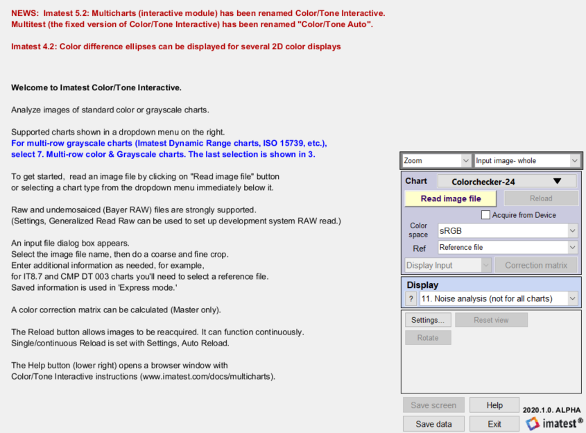
Color/Tone Interactive opening window with brief instructions
A standard Windows dialog appears with the chart type indicated in the title.
Open an image file by either pressing if the correct Chart type is displayed or by selecting a chart from the Chart type dropdown menu immediately above . The Chart dropdown has a two-tiered menu, which allows you to select color, multi-row grayscale, or linear grayscale charts. Color charts are shown below.
To calculate temporal noise, select either two files (for the Imatest-recommended difference method) or 4-16 files (for the ISO 15739 method). Details of the calculation are can be found here.
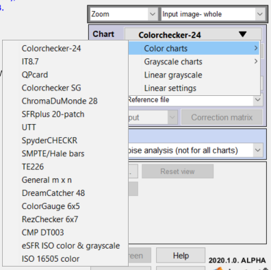
|
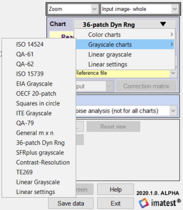
|
Supported charts (not all are shown below)
|
Select a chart to analyze by clicking on one of the entries in the Chart type popup menu described above or by clicking on if the correct Chart type is displayed. The button and popup menu (shown on the right) are highlighted (yellow background) when Color/Tone Interactive starts. Color/Tone Interactive and Auto support all charts shown and described below: | |
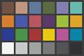
| The standard 24-patch X-Rite ColorChecker® Classic. ColorChecker charts (Classic and SG) are available in the Imatest store and from a great many suppliers worldwide. Images of both the 24-patch ColorChecker and SG can be found in Imaging-Resource.com camera reviews (in the samples section). Danny Pascale/Babelcolor's page on the ColorChecker contains nearly everything you want to know about the chart. Builds of Imatest 5.1 after May 2018 can read pre and post-2014 Colorchecker values from CGATS files posted on this page. |
|
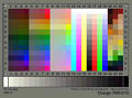
| The industry-standard IT8.7 chart. IT8.7 charts come in several formats (reflective and transmissive), available from Wolf Faust. A high-gamut version may be available from Hugo Rodriguez (website in Spanish). Reflective IT8.7/2 charts are relatively inexpensive. IT8.7 charts are usually printed on photographic paper or film (consisting of three dye layers). They must be used with reference files, which are available from manufacturer's websites. As of 2025, the IT8.7 is used infrequently, and we do not recommend it for new projects. |
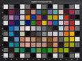
| The 140-patch X-Rite Colorchecker SG (Imatest Master & IS-only), which has a semigloss (SG) surface. It contains a 6x4 patch area in the upper-middle that is similar to the 24-patch Colorchecker, except that the colors are more saturated. Available from the Imatest Store. Imatest can read pre and post-2014 Colorchecker SG values from CGATS files posted on this page. | |
| Linear grayscale step charts (consisting of a single row of patches) such as the Kodak/Tiffen Q-13/Q-14 (inexpensive and widely available) or the Stouffer T4110 (Dmax = 4.0). Both reflection and transmission charts are supported. Charts with circular patterns (shown below) are preferred because they're less susceptible to errors from lens light falloff (vignetting). Other stepcharts are discussed in Using Stepchart. | |
|
|
Reflective Multi-row grayscale charts (Imatest Master-only): These charts are less susceptible to measurement errors from light falloff than linear charts.
Left: ISO-15739 Right: ISO-14524 | |
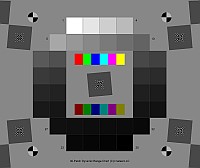 |
Transmissive Multi-row grayscale charts for Dynamic Range measurements (Imatest Master-only)
Right: Contrast Resolution Chart - Also for Contrast detection probability (CDP) | |
|
|
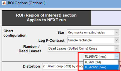
TE269 For Dynamic Range measurements. You can choose between the original version and the newer TE269V2 or V3 (which have the same geometry as the Imatest 36-patch DR chart, but different numbering) in a dropdown menu in the Chart configuration area of the ROI Options window. Three reference files are available, derived from data on the manufacturer's website: TE269A | TE269B | TE269C | |
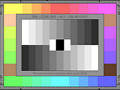 | DSC Labs ChromaDuMonde 28/28R widely used in the cinema and broadcasting industries for calibrating cameras. Useful with the vectorscope display. Imatest Image Acquisition features auto-refresh for full vectorscope functionality. | |
|
| The Universal Test Target (crop shown on right) is primarily designed for testing scanners. Color/Tone Interactive can analyze the 9x3 color pattern to the left of center (with the 9 light regions at the bottom) as well as the 20-step grayscale step charts (which have step increments of L* = 5). When the stepchart is analyzed (using 6. Stepchart (linear)), Ref (Reference file or data source) should be set to L* = 95:-5:5,1 (20-step UTT). | |
|
General mxn charts (4x12 shown on the left). Any chart with an m×n grid can be analyzed. You must specify the grid size by clicking Settings, then entering the number of rows (m) and columns (n) on the lower-right of the Settings window. We recommend doing this after opening Color/Tone Interactive, but before reading the image. You must also enter a CSV or CGATS file with reference patch settings (typically L*, a*, b* values, one set per line). If you have a spectrophotometer you can create a custom reference file (CGATS format) using techniques described in Measuring test chart patches. | |
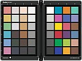 | SpyderCHECKR (8x6) A small chart that competes with the Colorchecker. Should be oriented as shown. If you want to measure only half the chart (say, left or right), you'll need to create a reference file with L*a*b* data available here. | |
|
Reference data for for the version with glossy grayscale patches (max density = 2.42) is built into Color/Tone. You can download reference file for the chart with matte grayscale patches (max density = 1.485) here. The patches are mounted on aircraft-grade anodized aluminum and are set below the top surface to help protect from damage. Nano patch sizes are 1/8” x 1/8”; 11/16” x 13/16” x 0.060” thick overall. Micro patch sizes are 1/4” x 1/4”; 1 -3/8” x 1-5/8” x 0.060” thick overall. | |
| ||
| Other charts: SFRplus 20-patch color, SMPTE/Hale Color Bars (6 patches), Image Engineering TE226 (9x5). We occasionally add charts on customer request. | ||
If the image is the same size and type as the previous image analyzed by Color/Tone and if Automatic region detection has not been selected (available for a limited number of charts), you'll be asked if you want to use the same ROI (region of interest).
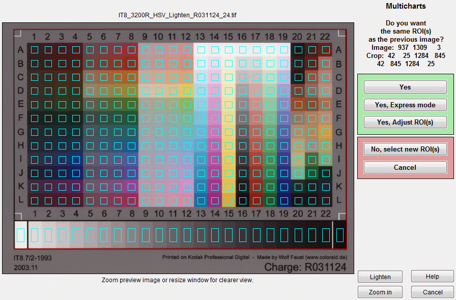
ROI repeat dialog shown with IT8.7 chart
If the image is not the same size and type, or if you answer No, a coarse cropping box appears. The initial crop doesn't have to be precise: you'll have a chance to refine it shortly. The crop box can be enlarged or maximized to make the selection easier.
- For either of the ColorCheckers (24-patch or SG), leave a margin around the sides slightly smaller than the spacing between patches.
- For grayscale step charts, select the entire chart (all patches), choosing boundaries that give even patch size. (The white patch on the Q-13 and Q-14 is larger than the rest.)
- For IT8.7 charts, select an area that includes the boundaries around the color chart and the entire grayscale (the red rectangle in the fine adjustment box below).
Special settings for linear grayscale charts
If you selected Linear grayscale (6. Grayscale Stepchart (linear*) and clicked No, select new ROI(s) in the ROI repeat window (if it appears)), the box shown on the right appears. Select the chart type (which specifies the density step) and the number of patches (between 6 and 41). Kodak/Tiffen Q-13/Q-14 charts have 20 patches; the Stouffer T4110 (a transmission chart with a density range of 4.0) has 41. For the Universal Test Chart (UTT) L* = 95:-5:5,1 (20-step UTT) and 20 patches should be selected.
*Linear charts have a single row of patches.
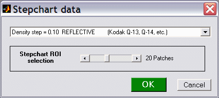
Stepchart type (reflective/transmissive, density step)
To correctly analyze the 36-patch High Dynamic Range (HDR) chart you must enter the individually-measured reference file.
Once you've made the rough crop, the fine adjustment box appears. The original crop is displayed as the red rectangle. The patch regions to be selected are the small cyan squares or rectangles. This dialog box can be enlarged or maximized to facilitate the adjustment. It offers numerous options.
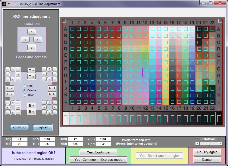
- The entire ROI can be moved ( , upper-left).
- The top, bottom, left, or right sides can be moved ( , middle-left).
- Corners can be moved individually (any of the 8 buttons in each of the four corners, middle-left).
- Pixel values for the four corners can be entered (X(tl), Y(br), ..., where tl = top-left, br = bottom right, etc.). The origin is the upper-left. Be sure to press the key after entering a value.
- You can choose between Fine and Coarse movement (1 or 5 pixels of movement per click).
- The display can be zoomed out or in.
- The display can be lightened to view the dark regions more clearly.
- For some charts (those with relatively large patches) a Fill factor (linear) slider in the gray area above the button specifies the relative size of the squares. Its default value is 0.5. Smaller values can be used where lens distortion or pattern alignment makes alignment difficult.
- The distortion slider allows highly distorted images (barrel or pincushion) to be analyzed.
When you have completed the fine adjustment, click one of the buttons on the bottom of the window. If you click , an additional dialog box may appear. For example, for the IT8.7 chart it will ask for the required reference file. Some of the entries in the input dialog boxes, like color space, can be changed later. If you click , it will go directly to the Color/Tone window, using saved (most recent) values. For example, it saves the IT8.7 reference file name.
To save ROIs for use in future runs or to retrieve ROIs saved in past runs, follow the instructions in How to save and retrieve region selections. The ROIs are for the individual chart (Colorchecker, Contrast Resolution, etc.), not for Color/Tone as a whole.
Reference files
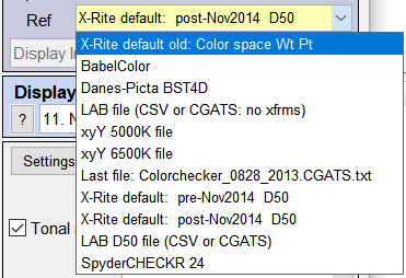 Most charts allow reference files to be entered using the Ref. dropdown menu in the image area on the right of the Color/Tone window, below the Color space box. (IT8.7 and 36-patch Dynamic Range charts require them.) The available settings depends on the chart type. The previous file is generally available in the dropdown list. Here is a summary of the available reference sources.
Reference file selections for the X-Rite Colorchecker,
which has more choices than any other chart.
If you enter LAB or xyY file, Imatest requests the file name.
| You can obtain the current reference data from the Color/Tone window by pressing File (dropdown menu on the upper-left), Copy L*a*b* reference to clipboard, or File, Copy density reference to clipboard. |
| Chart | Default values | Options (data from files) |
| X-Rite ColorChecker (24-patch) | Default values from X-Rite, BabelColor, or Danes Picta (a chart with the same geometry but different colors). See Notes 1 and 2 below. | L*a*b*, xyY D50, or xyY D65 files in CSV format. |
| 36-Patch Dynamic Range charts Contrast Resolution chart | 36 densities from 0.1 to 3.6 in steps of 0.1. This is the target for the single layer chart, but it is only a very rough approximation. A density file is required for valid measurements on 36-patch DR charts and recommended for the Contrast Resolution chart. | A Density CSV file (one value per line) is preferred, but a L*a*b* CSV file (three values per line) can be used. |
| IT8.7 | Requires a reference file in IT8.7 format, available from the chart manufacturer, generally available on their websites. | — |
| Rezchecker | You can use the standard default reference or NIST-traceable measurements provided by ISA. These measurements are in a difficult-to-use XLS/CGATS file format. To use this data, open the file in Google sheets (which can be done directly in Gmail) or in Excel. Select the 30 rows representing the patches and the 3 column representing LAB L, LAB A, and LAB B, and copy them into the clipboard. Past into a text editor and save the file (with txt or csv extension). Reference data for for the chart version with glossy grayscale patches (max density = 2.42) is built into Color/Tone. The reference file for the version with matte grayscale patches (max density = 1.485) can be downloaded here. | |
| X-Rite ColorChecker SG | Default values from X-Rite (L*a*b* D50); See Notes 1 and 2 below. | L*a*b*, xyY D50, or xyY D65 files in CSV format. |
| Stepchart (linear) | Even density steps of 0.1, 0.15, 0.20, or 0.30. For the UTT only, L* = 95 to 5 in steps of -5 for the first 19 steps and 1 for step 20. (20-step UTT) should be selected. | an ASCII density reference file with one density value per line can be entered. |
|
Note 1: Several of the default reference values are derived from L*a*b* D50 values, i.e., L*a*b* values acquired under D50 illumination. When the color space has a different reference temperature (sRGB and Adobe RGB both have D65) a Bradford transformation is applied, resulting in a small change in the L*a*b* values. This is rarely a significant concern if you're making images under a different illuminant: if the white balance algorithm is working properly, it should transform image colors to the appropriate values for the color space. Note 2: Builds of Imatest 5.1 after May 2018 can read pre and post-2014 Colorchecker Classic and SG values from CGATS files posted on this page. | ||
Except for the IT8.7, reference files must be in CSV (comma-separated) or CGATS format. CSV files can be opened and edited in Excel. Color CSV files (L*a*b*, xyY D50, and xyY D65) have three entries per line; density files have have one entry per line.
Here is an example of an L*a*b* CSV file.
CSV format (comma-separated variables).
The format is the same for xyY files.
Added spaces are for visual clarity (readability)-only.
28.778, 14.179, -50.297
65.711, 18.13, 17.81
51.038, -28.631, -28.638
51.935, 49.986, -14.574
81.733, 4.039, 79.819
42.101, 53.378, 28.19
If you have a spectrophotometer you can create a custom reference file (in the CGATS format, supported by Imatest 3.10+) using techniques described in Measuring test chart patches.
|
The color reference for a test chart contains CIELAB (device-independent L*a*b*) values for each patch of the chart. It can be
Questions frequently arise regarding the color temperature used to (1) measure the patches for the reference file, (2) measure camera color accuracy from a chart image, and (sometimes forgotten), and (3) built into the color space used by the camera under test. (All interchangeable files have a color space associated with them, implicitly or explicitly.) Patches are measured with a light source with a known color temperature, typically 5000K. Color spaces have a illuminant white point. sRGB (the widely used internet Windows standard) has a 6500K illuminant white point and a D50 (~5000K) ambient (viewing environment) white point. Wikipedia does little to resolve the confusion, but the 6500K illuminant white point is the chief property of the file. A Bradford transform is typically applied to convert the 5000K measurement to the 6500K color space illuminant white point.. A frequent question is, "Is a special reference file needed for measuring charts with illuminants different from the color space white point (typically 6500K)?" The question is important because Imatest measurements (and indeed almost all camera operation) can be made with a wide variety of color temperatures, ranging from 2400K for incandescent lights to >10000K for some daylight conditions. The quick answer is "No". The standard reference file should be used. The raw image is often transformed in the camera by an algorithm that estimates the illuminant color temperature, then applied a Color Correction Matrix to the image to white balance it and correct the colors. The CCM can also be applied to an uncorrected image by Imatest. |
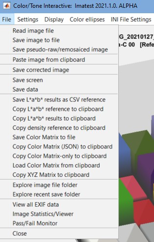 Obtaining the color reference values
In Color/Tone Interactive you can perform a number of operations that relate to the reference file using the File dropdown menu, shown on the right.
The operation of interest here is Copy L*a*b* reference to clipboard. This shows the currently selected reference, whether it’s a standard or custom file. You can also save it as a named file for future use as a reference— perhaps for a “gold standard”. Here are the first three values for the post-Nov 2014 X-Rite Colorchecker default values.
37.31 13.39 14.58
64.37 18.05 17.05
49.62 -1.162 -22.16
…
For grayscale patterns, Copy density reference to clipboard is available in the File dropdown menu on the right.
The Color/Tone Interactive window
After the image file has been entered, the most recent Chart view is displayed. The 2D a*b* view (ideal and input values on the CIELAB a*b*) is shown below.
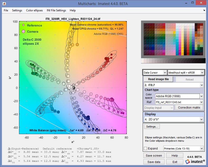
The main display image is on the upper left. Color differences are summarized below this image, except when the Probe is turned on (available for the pseudocolor and split color displays). The various ?E* and ?C* values are described in in Wikipedia. A thumbnail image of the chart is shown on the upper right. Available options are described below. The remainder of the right side is the control area.
The Zoom/Rotate 3D/Data Cursor dropdown menu, just below the upper-right thumbnail, determines the action when you click on the image.
| Zoom | Click on the image or select an area to zoom into. Double-click to zoom out. | 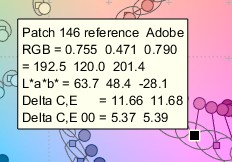 |
| Rotate 3D | Rotate 3D images by clicking and dragging the mouse. Zoom is activated for all other (2D) images. | |
| Data Cursor | Display a data cursor (shown on the right) for several displays including 4. 2D a*b*, 5. xy Chromaticity, and 6. u'v' Chromaticity. When you click on Reference or Camera symbols, you get a Data cursor with patch information: RGB and L*a*b* values (different for the reference and camera) and several color difference metrics. |
The dropdown menu to the right of the Zoom/Rotate 3D/Data Cursor menu controls the display of the thumbnail image on the upper-right. The first two selections use the actual image. The rest use synthesized (reference and camera) patches.
| Input image- whole | Shows entire input image | |
| Input image- crop | Shows the cropped input image (all patches) | 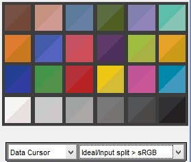 |
| Ideal/Input split > sRGB | shows a split view of the ideal/camera patch values mapped to sRGB, which is similar to typical monitor color spaces. This is the default (recommended) setting (shown on the right for the X-Rite ColorChecker). | |
| Ideal/Input split patches | shows a split view of the ideal/camera patch values with no gamut mapping. Colors will not be accurate for large gamut color spaces | |
| Input > sRGB monitor | displays the input image mapped from its native color space to sRGB, which is similar to typical monitor color spaces | |
| Input patches | displays the input image with no gamut mapping. Colors will not be accurate for large gamut color spaces | |
| Ideal > sRGB monitor | displays the ideal image mapped from its native color space to sRGB, which is similar to typical monitor color spaces | |
| Ideal patches | displays the ideal image with no gamut mapping. Colors will not be accurate for large gamut color spaces | |
Image area
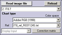
The pale blue box on the right is the image area. It includes the button (and button for Imatest Image Acquisition-only), the Chart type dropdown menu (described above), entries for image properties, and color correction matrix functions .
(Imatest Image Acquisition-only) reacquires the image from a device or video stream (depending on how the image was originally acquired) or reloads it from a file.
Color space allows the input file color space to be selected. This color space is also used as the target for calculating the Color Correction Matrix (CCM). The color space is automatically read into Color/Tone from the EXIF data when ExifTool has been selected in Options II; otherwise it must be entered manually. Several color spaces are available. The first six are primarily for still images. Most of the rest are for video/cinema. See the Wikipedia RGB Color Space page and brucelindbloom.com for overviews.
| sRGB | The default space of Windows and the Internet. Limited color gamut based on typical CRT phosphors. Gamma = 2.2 (approximately), White point = 6500K (D65). |
| Adobe RGB (1998) | Medium gamut, with stronger greens than sRGB. Often recommended for high quality printed output. Gamma = 2.2, White point = 6500K (D65). |
| Wide Gamut RGB | Extremely wide gamut with primaries on the spectral locus at 450, 525, and 700 microns. One of the color spaces supported by the Canon DPP RAW converter. 48-bit color files are recommended with wide gamut spaces: banding can be a problem with 24-bit color. Gamma = 2.2, White point = 5000K (D50). |
| ProPhoto RGB | Extremely wide gamut. Gamma = 1.8, White point = 5000K (D50). |
| Apple RGB | Small gamut. Used by Apple. Gamma = 1.8, White point = 6500K (D65). |
| ColorMatch RGB | Small gamut. Used by Apple. Gamma = 1.8, White point = 5000K (D50). |
| Rec. 709 Legal | HDTV color space. Gamut similar to sRGB. D65 White point. Allowable pixel levels 16-235 |
| Rec. 709 Full | HDTV color space. Allowable pixel levels 0-255 |
| ACES | Academy Color Encoding System. Gamma = 1 (linear). Extremely wide gamut covers all visible colors with primaries outside the visible spectrum. D60 White point. File data stored as half-precision floating point (OpenEXR format). |
| Rec. 2020 Legal | UHDTV color space. Much larger gamut than Rec. 709. D65 White point. Allowable pixel levels 16-235 |
| Rec. 2020 Full | UHDTV color space. Allowable pixel levels 0-255. |
| DCI-P3 | Digital cinema projection color space. 25% wider gamut than sRGB, covering most reflective surface colors. Gamma = 2.6. |
| Display P3 | Used in the iPhone 8. Same gamut as DCI-P3, but gamma is approximately 2.2 (same as sRGB). May be a part of the new Apple HEIF file format, intended to replace JPEG. This is new information (as of late 2017). Reliable information is hard to come by. |
Danny Pascale's A Review of RGB Color Spaces is recommended for readers interested in an in-depth explanation of color spaces.
Ref lets you select source for the reference (ideal) chart values, as described above. The dropdown menu contents depends on the chart type. For the 24-patch ColorChecker and the ColorChecker SG you can select either standard chart reference values or you can read in values from data files (Imatest Master and Image Sensor) in CSV or CGATS formats. Values for the two ColorCheckers have been supplied courtesy of X-Rite.
calculates the Color Correction Matrix (CCM). Prior to calculating the CCM you should make sure settings (linearization, etc.) are correct by clicking on or clicking Settings (dropdown menu), Color matrix and other settings... After has been pressed it changes to , highlighted with a yellow background. The correction matrix cannot be recalculated until a property of the image (new image, color space, reference file, or color matrix setting) changes. The Display input (or Corrected) dropdown menu, immediately to its left, is enabled. More details on using the Color Correction Matrix can be found here.
Display selection menu and area
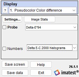
- Pseudocolor color difference. Shows the difference between the ideal and input color patches using any of several metrics. The pseudocolor scale is shown adjacent to the image (below, right). Probe is available for this display. Not the most useful display
- 3D color difference (with split colors).
- Split colors: ideal/input. Shows the patches split so that the ideal and input values are displayed in the upper left and the lower right or each patch region, respectively. Probe is available for this display.
- 2D a*b*.
- xy chromaticity.
- u'v' chromaticity.
- Black & White density.
- 3D L*a*b*. Shown on the right. L*a*b* coordinates can be difficult to visualize when viewed from a single angle. It needs to be rotated to be useful.
- EXIF data and Color matrix. Shows EXIF data if available and the color correction matrix if it has been calculated.
- Vectorscope preview.
- Noise analysis (not for all charts). A huge variety of noise, Signal-to-Noise Ratio (SNR) and Dynamic Range results are available, including ISO 15729 and CPIQ (Camera Phone Image Quality) results. See Color/Tone/eSFR ISO noise for more details. Not available for charts with tiny patches, like the IT8.7 and ColorChecker SG.
- Display image. Many options are available including display single channel, boosted colors, and lightened image.
- Read - color-correct - Save image. Can be used after CCM has been calculated to apply the Color Correction Matrix to any image. The corrected image can be saved.
- 2D CbCr (from YCbCr).
- HS (Hue-Saturation) from HSV.
- HS (Hue-Sat) from HSL.
The Display area, immediately below the Display selection box, contains display options. The contents, which depend on the display selection, are described below in the sections for the individual displays.
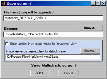
(shown on the right) saves a snapshot of the current display (the entire Color/Tonescreen) as a PNG file (a widely-used losslessly compressed format). It also allows you to immediately view the snapshot so it can be used a reference for comparing with other results.
File name and Directory at the top of the window set the location of the file to save.
When you check the Open window in an image viewer... box, the current screen will be opened either the system default viewer (if the box under Image viewer is blank) or a viewer/editor of your choice (if the box contains the path name to the viewer/editor). I recommend using Irfanview, which is fast, compact, free, and supports an amazing number of image file formats. Its normal location in English language installations is C:\Program Files\IrfanView\i_view32.exe.
Saves the key data in CSV and XML formats. This includes the input R, G, and B values, the input and reference L*, a*, b* values, and several of the color difference metrics.
opens this web page in an HTML browser window.
terminates Imatest Color/Tone, but the Imatest main window is still available.
More settings
Clicking the button that appears in the Display area (for many displays) or clicking Settings (dropdown menu on top), Color matrix and other settings... or ISO speed, noise, mxn chart... opens the window shown below.
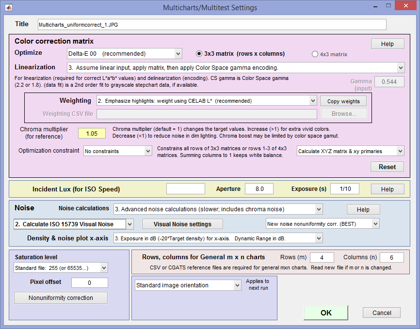
| Color correction matrix | Settings for the CCM calculation are described in the Color Correction Matrix page |
| Incident Lux | Must be manually entered for ISO Sensitivity (Exposure Index) calculations. Aperture and Exposure (s) are normally obtained from EXIF data, but may be entered manually if the EXIF data is absent. |
| Noise | Settings are described in the Color/Tone/eSFR ISO Noise page. |
| Rows, columns for General mxn charts | Select number of rows and columns for general mxn (rectangular) charts. A reference file is required for this chart selection. |
| Saturation level |
The maximum pixel level for the input image, corresponding to saturation level, used for normalizing image data for certain calculations. Standard file: 255 (or 65535...): The saturation level is automatically set based on the data type and container size of the image data. This is the default setting. The image file is assumed to have standard bit depth (e.g., 8, 16, or 32 -bit data) and standard saturation level. For example, for standard 8-bit image data, saturation level will be set to 255. For a 16-bit image, saturation level will be set to 65535, and for a 32-bit image, saturation level will be set to 4294967295. ITU-R Rec. 601 (BT. 601: 235): The saturation level is set to 235. Maximum detected patch level: The saturation level is set to the maximum detected value from the patch regions in the image. Can be useful if the image data is of nonstandard bit depth (e.g., 12-bit data stored in a 16-bit container) or if there is a custom saturation level, so long as the image is exposed to saturate the brightest patches. Manually-entered saturation level: The saturation level is set to the value entered by the user. Can be useful if the image data is of nonstandard bit depth or if there is a custom saturation level. For example, for an image that has 12-bit data stored in a 16-bit container, enter 4095 as the saturation level (2^12 - 1 = 4095). |
| Pixel offset | Enter the pixel offset to subtract from the data. Pixel offsets are not uncommon: they cause a premature flattening of Density curves. |
| Nonuniformity correction | Allows you to correct for nonuniform illumination using a separate flat field image taken under identical conditions. Opens the Nonuniformity correction window described in Nonuniformity Correction in grayscale and color chart modules. |
| Image orientation | (Applies to next read) Select among Standard image orientation, Mirror (H-flip), Mirror (V-flip), Rotate 180 degrees. |
Dropdown menus File Settings Color ellipses INI File Settings Help
The Dropdown menus at the top of the Color/Tone window are used for a large variety of utilities and settings.
| File |
| ||||||||||||||||||||||||||
| Settings |
| ||||||||||||||||||||||||||
| Color ellipses |
| ||||||||||||||||||||||||||
| INI File Settings | INI file utilities, described in INI File Utilities. | ||||||||||||||||||||||||||
| Help | Open online Help pages— instructions relevant to Color/Tone. |
Displays and options
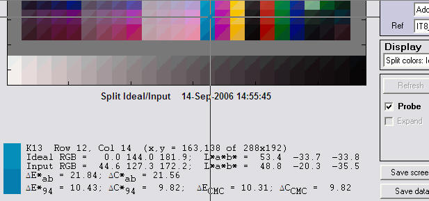
1. Pseudocolor Color differenceShows the difference between the ideal and input color patches using any of several metrics using a pseudocolor color map. If a color correction matrix has been calculated, the difference between the ideal and corrected patches are shown at the bottom. The pseudocolor scale is shown adjacent to the image. (Checkbox; Pseudocolor and Split views) turns on the probe, illustrated below. When the probe is on, you can probe any patch by clicking on it. The probe data (for the individual patch), shown below the split display, includes a small image of the ideal and input patch colors, ideal and input RGB and L*a*b* values, and several ?E* and ?C* color difference metrics. (Corrected colors are used if a color correction matrix has been calculated and Display corrected has been selected.) The probe is turned off by clicking outside either of the images. ?E*ab, the geometric distance in L*a*b* space, is the most familiar, but ?E*94, which is lower for chroma differences in highly chromatic colors (with large a*2 + b*2), is a better measure of visual color difference. ?E*00 is the most accurate metric (based on an exceedingly complex designed-by-committee equation). More detail on color difference equations can be found here and in Wikipedia. |
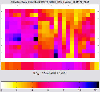 Pseudocolor display for IT8.7 Pseudocolor display for IT8.7 |
|
Probe illustration Split display for IT8.7 illustrating Probe (available for pseudocolor and split color displays) (Popup menu to the right of the Probe checkbox; also in 3D Color difference) Contains a list of color metrics (mostly difference metrics) including ?E*ab, ?C*ab, ?E*94, ?C*94, ?E00, ?C00, ?L*, ?Chroma, ?|Hue distance| , ?(Hue angle) , Chroma (input) and Chroma (output). Numbers (checkbox) displays numbers in the middle of patches if checked. Color map (Popup menu) allows you to select the color map. The WYRMBK color map shown goes from White - Yellow - Red - Magenta - Blue - Black. | |
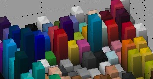
2. 3D Color difference (with split colors)Uses the height of the patches to display the difference between the ideal and input colors. Any of several metrics (?E*ab, ?C*ab, ?E*94, ?C*94, ?E*CMC, ?C*CMC, ?E*00, ?C*00, ?L*, ?Chroma, ?|Hue distance|, ?Hue angle, Chroma (input), Chroma (output)) can be chosen. The faces show split colors: reference (upper-left)/input (lower-right). This allows you to compare visual color differences with standard color difference metrics. Can be zoomed and rotated. You can use this display to correlate ?E and ?C metrics with visual color differences. None of the metrics are perfect! The visual difference between the reference and input is often lower than the indicated differences because the color space and monitor gamuts (often sRGB) may be lower than the original chart gamut, especially for cyan and blue. (Toggle button; short for Auto rotate) starts rotating the image. Rotation is quite slow; it may be less useful than the 3D L*a*b* plot (below). The image continues to rotate until the next time you press the button. It's best to turn off rotation before switching to other views. Light (Checkbox) Illuminates the figure to make the sides darker. Checked (On) recommended. Color difference type (Popup menu) Described above under Pseudocolor display. Background lightness (Slider) sets the background gray level. Invert (Checkbox) inverts the up-down orientation of the 3D plot. |
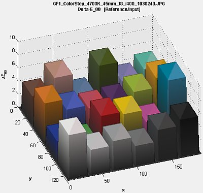 3D Color difference display for Colorchecker |
3. Split colorsDisplays a synthesized chart image with each patch split so the ideal value is in the upper left and the input (measured) value is in the lower right. If a color correction matrix has been calculated, corrected colors are shown at the bottom. (Checkbox) is the only option. Described above under Pseudocolor display. Numbers (checkbox) displays numbers in the middle of patches if checked. |
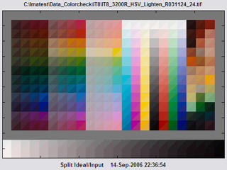 Split Color display for IT8.7 |
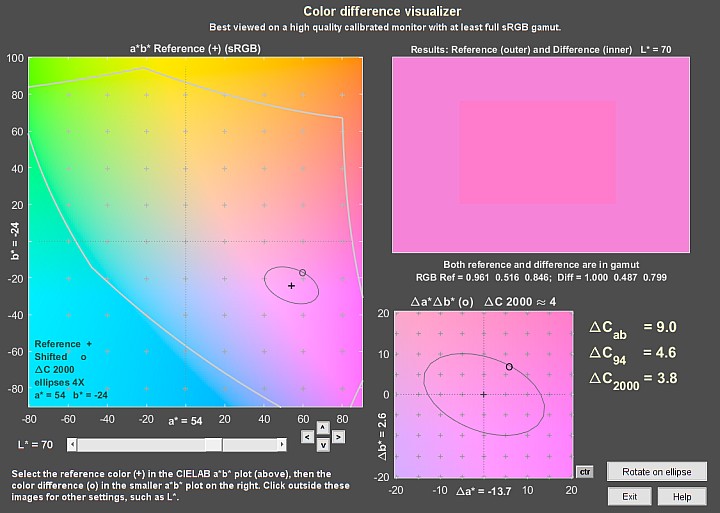
4. 2D a*b*Displays patch values on the CIELAB a*b* plane. Ideal values are displayed as squares; Input values are displayed as circles. Color difference ellipses (representing ?Cab, ?C94, or ?C2000 can be displayed. A Color Difference Visualizer (separate from Color/Tone Interactive) has been added so you can interactively examine the appearance of color differences. Expand (Checkbox; 2D a*b*, xy chromaticity, u'v' chromaticity, and 3D L*a*b*) Zoom in so the data fills the image. (Popup menu in the lower right of the Display area; also in xy chromaticity, u'v' chromaticity, and 3D L*a*b*) selects the region of the chart to display. For the IT8.7 and ColorChecker SG charts only. Avoids clutter from the large number of patches in these charts.
|
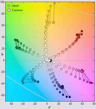 2D a*b* display for IT8.7
|
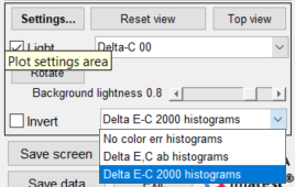
Histograms (available with plots 1-4: Imatest 2021.2+)
The histograms are useful for comparing color errors without and with a color matrix (CCM) applied. | 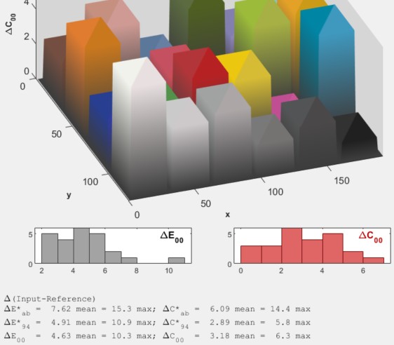 ΔE00 & ΔC00 histograms in plot 2 ΔE00 & ΔC00 histograms in plot 2 |
5. xy and 6. u'v' ChromaticityDisplays the xy and u'v' Chromaticity diagrams, which separate the visible and invisible color values into colored and gray regions. Ideal values are displayed as squares; Input values are displayed as circles. Color difference ellipses (representing ?Cab, ?C94, or ?C2000 can be displayed. The u'v' Chromaticity diagram, which is more perceptually uniform than the more familiar xy diagram is illustrated on the right. (Checkbox) Turns the wavelength display (400-700 microns) on the periphery of the locus of visible colors on or off. (Popup menu to the right of Wavelth) selects between normal color (about as good a representation as is possible on a monitor) and lightened color (slightly easier to see the patch values). (Checkbox) Zoom in so the data fills the image. (Popup menu in the lower right of the Display area) Described above under 2D a*b* display. |
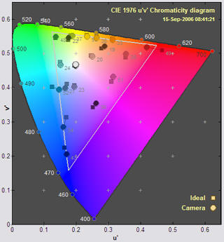 u'v' display for ColorChecker SG |
7. Black & White densityShows the grayscale response curve. Available for all currently-supported color charts because all of them contain grayscale regions. (Popup menu) allows you to select one of several B&W displays.
When the B&W density plot is displayed, you can enter the incident lux level into a box in the Display area on the lower right of the Color/Tone window. If the value is a positive number (not blank or zero) ISO Sensitivity will be calculated and displayed on the plot. |
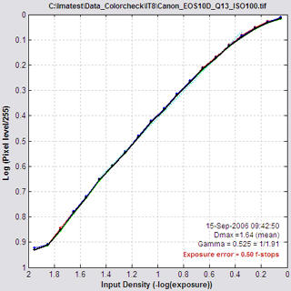 Log pixels vs. input density for Q-13 |
8. 3D L*a*b*Displays patch values in 3D CIELAB L*a*b* space with a wireframe representing the boundaries of the selected color space. Ideal values are displayed as squares; Input values are displayed as circles. Can be zoomed and rotated; you need to rotate it to be able to visualize patch locations. (Popup menu) Turns wireframe on, off, or on with minimal (coarse) grid. (Toggle button; short for Auto rotate) starts rotating the image. This provides a better visual indication of the color locations. The image continues to rotate until the next time you press the button. It's best to turn off rotation before switching to other views. (Slider; default = 1) sets the wireframe transparency.Reducing transparency below 1 differentiates patches outside and inside the wireframe gamut boundary. Results are not reliable: patches near the boundary don't always appear as they should. (Slider) sets the background gray level. (Popup menu in the lower right of the Display area) Described above under 2D a*b* display. (Checkbox) Zoom in so the data fills the image. |
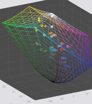 3D L*a*b* display for ColorChecker 3D L*a*b* display for ColorChecker |
10. Vectorscope (not in Studio)Duplicates the display of hardware vectorscopes, used for adjusting and calibrating broadcast and cinema cameras. It is designed to work optimally with the DSC Labs ChromaDuMonde 28 chart. (Other DSC charts will be added as customer demand warrants.) There are several display options, including background color, reference and input display color. Light input colors (circles) and dark reference colors (squares) are shown on a dark background. HDTV, SDTV (similar to YCbCr below), and NTSC/PAL vectorscope patterns can be displayed. The recommended color space for these signals is sRGB. For now the vectorscope omits the standard target rectangles because the RGBCMY primaries in the CDM chart are different from the standard color bars. This image is a preview of a full-featured vectorscope function that will be included in an upcoming broadcast/cinema version of Imatest that continuously refreshes frames from a video stream using the button instead of reading individual images from files. |
|
11. Noise analysis (for charts with large enough patches)Color/Tone supports a variety of noise and SNR (Signal-to-Noise Ratio) analyses, including plain pixel noise, chroma noise, CIELAB (L*a*b*) noise, Dynamic Range analysis, Photon Transfer Curves (noise or SNR as a function of Digital Number (DN) for Simatest, and ISO 15739 visual noise. These measurements are for the grayscale patches. The measurements include a set of measurements for all patches (color as well as grayscale) that is meaningful for undemosaiced raw images (i.e., no tonal response curve or color matrix applied). In such systems, noise is proportional to a constant plus the square root of the pixel level. This measurement allows you to determine the sensor dynamic range (using a fairly reliable extrapolation). See Color/Tone noise for more detail. | 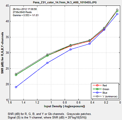 SNR measurement SNR measurement |
12. Display imageThe image can be displayed to verify the region settings and to explore the patche images (under a variety of conditions-- normal view, intensified color, lightened, etc.). Options: Image display (dropdown menu; title not displayed due to space limitations) allows you to select Original image, individual channel (R, G, B, Y, mean), chroma-boosted image, lightened image (several versions), etc. Useful for finding issues in the image as a whole or in individual patches. Display patch ROIs (checkbox) Turns red ROI rectangles on or off. Crop (checkbox) If Crop is checked, a dropdown menu is opened, just to the right of the Crop checkbox, that allows you to select Whole crop or the individual patch. | 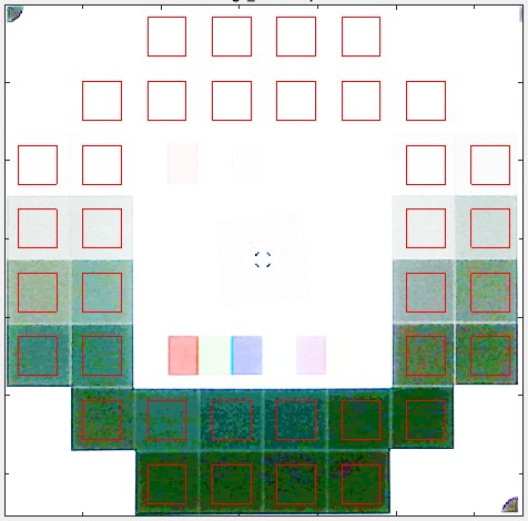 |
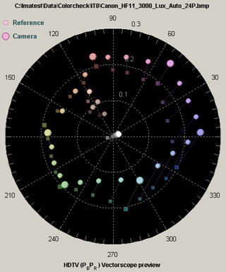 Vectorscope preview
13. Read – color correct – Save image
Once a color correction matrix has been calculated, the matrix can be used to correct arbitrary images. To do so, select 11. Read - color correct - save image in the Display box on the right of the Color/Tone window. The initial display on the left side contains the message, Press "Read image to correct", then press "Save corrected image" if it looks OK., the color correction matrix and statistics, and two buttons: and .
In the case shown on the right, a (digital) CC20C (cyan) filter was applied to both the Colorchecker and Gallery image. The correction matrix was calculated for the filtered Colorchecker, then the filtered Gallery image (shown uncorrected on the top) was read in. The corrected image is shown on the bottom.
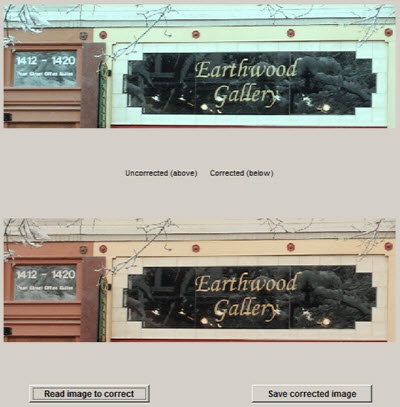 Color correction on an arbitrary scene
14. YCbCr plot
Displays results on the CbCr plane of YCbCr color space. Similar to the Vectorscope plot with SDTV selected.
Expand (Checkbox; available in several 2D plots) Zoom in so the data fills the image.
15. HS (from HSV) and 16. HS (from HSL) plots
Displays H (Hue) angle and S (Saturation) radius for HSV and HSL color representations, respectively. These representations are relative to the color space gamut boundary, which is located at radius = S = 1, i.e., they are not device-independent.
Expand (Checkbox; available in several 2D plots) Zoom in so the data fills the image.
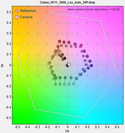
YCbCr plot
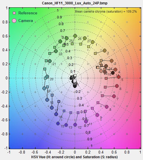 H (Hue) and S (Saturation) from HSV H (Hue) and S (Saturation) from HSV | 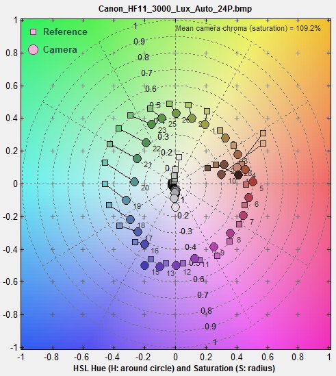 H (Hue) and S (Saturation) from HSL H (Hue) and S (Saturation) from HSL |
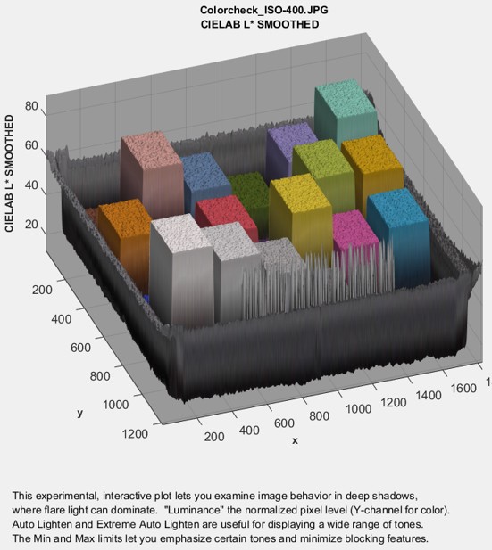
17. 3D Image Surface plot
The surface height is the luminance (Y-channel) of the image.
分析颜色和灰度测试图表
在一个固定的、能够进行批量处理的模块中
Color/Tone Auto(以前称为 Multitest)包含了Color/Tone Interactive (以前称为 Multicharts) 、 Colorcheck和Stepchart中的所有计算。
“颜色/色调交互式”和“颜色/色调自动”模块现在可以测量时间噪声和信噪比。此次增强后,这两个新模块具备了旧版“阶梯图”和“颜色检查”模块的所有主要功能,但旧版模块不建议用于新项目。 |
使用 Color/Tone Interactive (原 Multicharts) ——对颜色和灰度测试图表进行交互式分析 使用颜色/色调自动功能——固定(可批量处理)分析颜色和灰度测试图 色彩/色调/eSFR ISO噪点– 包括色度噪点、传感器噪点(RAW)噪点和视觉噪点 动态范围– 概述,并提供指向 Imatest 计算动态范围的模块的链接。 颜色校正矩阵 (CCM)计算一个矩阵(通常为 3×3),用于校正图像颜色(通常来自 RAW 图像)。 |
介绍
Imatest™ Color/Tone Auto是一款色彩/色调自动分析软件,它使用固定界面批量处理图像,可分析各种测试图表的图像,评估其色彩准确度、色调响应、噪声、信噪比 (SNR) 和ISO 感光度。该软件能够测量各种光照条件和场景下的白平衡和色彩响应,并可显示单色图表(或彩色图表中的单色部分)的色调响应。此外,它还能计算色彩校正矩阵。
Color/Tone Auto可以分析Color/Tone Interactive支持的所有图表,并生成大部分结果图。它还集成了Colorcheck和Stepchart模块的所有重要功能:操作方式类似,但能够分析更多图表并显示更多结果。
一套完整的图表及其使用指南都在其中。
颜色/色调测试图表参考及指南
| 24个补丁 颜色检查器 | IT8.7 | 对比度分辨率 | Colorchecker SG | |||||
三个版本 | Q-13/Q-14 以及其他 灰度 步骤图 | 颜色规 (微米、纳米等) | ||||||
ISO-15739 | 墨西哥将军 图表(L*a*b* 参考文件 必需的) | TE269,TE269V2 (2 个版本) | ISO-14524 | |||||
另附:SFRplus 20色块色卡、SMPTE/Hale 色条(6色块)、TE226(9x5)色卡 | ||||||||
支持的图表的更完整列表可在“颜色/色调 - 支持的图表”中找到。
入门
拍摄或扫描色卡时,注意均匀照明(误差±5%),并避免眩光。对于半光泽(SG)和光面色卡(例如反光的IT8.7和ColorChecker SG),眩光问题尤为突出。使用广角镜头时,眩光控制尤其困难。为尽量减少镜头光线衰减的影响,色卡通常不应充满整个画面。
《搭建低成本测试实验室》一文介绍了一种低成本的照明方案。为了测试白平衡,您可以在各种光照条件下拍摄场景中的色卡。小型版本的 ColorChecker 色卡(例如Passport 、 SpyderCheckr或 ColorGauge 色卡)尤其适合此用途。某些矩形色卡如果几何对称,可以旋转 ±90° 的倍数(例如两款 ColorChecker 色卡和 Kodak/Tiffen Q-13/Q-14,但不包括IT8.7,因为其上下两面不同)。
在运行“颜色/色调自动”功能之前,您应该选择要分析的图表类型。点击Imatest主窗口(如右图所示)中按钮右侧的按钮,或者点击“固定模块” > “颜色/色调自动设置” 。这些操作将打开“颜色/色调自动”设置窗口,如下图所示。 图表类型下拉菜单(位于“颜色/色调自动设置”窗口中,如右侧所示)包含所有可用的图表设置。 选择完成后,该设置将被保存并显示在按钮中,如右上图所示。 可以在此时或读取图像文件并选择感兴趣区域 (ROI) 后更改其他设置(除非您选择了快速模式)——但由于图表类型总是会影响下一次运行,因此在运行新的图表类型之前应该进行选择。 图表选择下拉菜单 运行“颜色/色调自动”之前应选择图表类型。 |  | |
图表类型(用于下次颜色/色调自动运行) 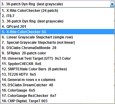 |
自动区域检测
这也是选择自动或手动区域检测的好时机,该功能位于“颜色/色调自动”设置窗口的底部,并且对允许自动选项的图表启用(最初是Colorcheck和36 色块动态范围图表,未来会有更多)。

运行颜色/色调自动功能—要启动颜色/色调自动功能,请运行Imatest ,然后单击按钮。此时将打开一个窗口,供您选择文件(或一批文件)。
要计算时间噪声,请选择两个文件(用于 Imatest 推荐的差分法)或 4-16 个文件(用于 ISO 15739 方法)。计算详情请参见此处。
如果您选择了手动 ROI 检测,在选择文件后,Imatest 会检查图像大小是否与最近运行的图像大小相同(它会保存多种尺寸的图像)。如果大小相同,系统会询问您是否要重复选择相同的感兴趣区域 (ROI):
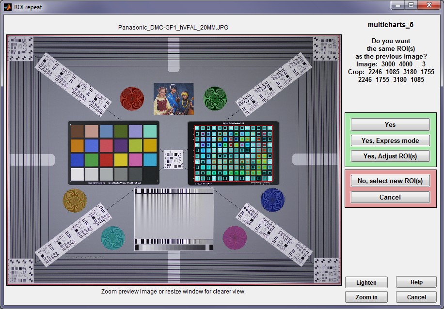
如果图像大小与之前的图像不同,或者您点击 ,则会弹出一个窗口,要求您选择区域。您可以通过在要分析的图表上从一个角到另一个角绘制一个矩形来完成此操作。不必担心区域是否完全精确——您可以对其进行微调。
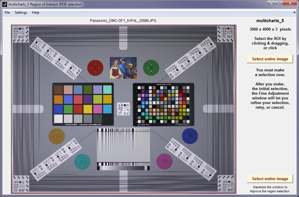
初步(粗略)区域选择。在图表上画一个从一个角到另一个角的矩形。
图片来自Imaging-resource.com (来自单个相机评测示例页面的多目标)。
在粗略选择后打开的精细选择窗口中,对选择区域进行更精确的调整。不同图表的内部方框可能有所不同。(注意:如果您选择了“自动 ROI 检测”选项,并使用支持自动检测的图表进行确认,则会显示此窗口。)
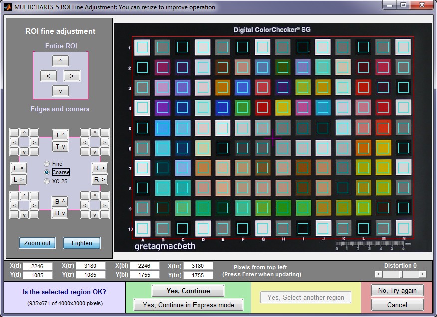
- 整个 ROI 可以移动(^ > v <,左上)。
- 顶部、底部、左侧或右侧可以移动(T^ Tv R> R< B^ Bv L> L<,中间向左)。
- 可以单独移动四个角(四个角中左侧的 8 个按钮中的任何一个)。
- 您可以输入四个角点的像素值( X(tl) 、 Y(br) 、…,其中tl代表左上角, br代表右下角,以此类推)。原点位于左上角。输入数值后请务必按回车键。
- 您可以选择精细、粗糙或超粗糙 (XC-25) 移动(每次点击移动 1、5 或 25 像素)。
- 显示内容可以缩小或放大。
- 可以调亮显示屏,以便更清楚地查看暗部区域。
- 对于某些图表(尤其是色块较大的图表),“失真”滑块左侧的“填充因子(线性)”滑块用于指定方块的相对大小。其默认值为 0.5。当镜头失真或图案对齐导致对齐困难时,可以使用较小的值。
- “失真”滑块允许分析高度失真的图像(桶形失真或枕形失真)。
完成微调后,单击窗口底部的按钮之一。如果单击 ,则会打开如下所示的“颜色/色调自动”设置窗口。如果单击 “颜色/色调自动”功能将运行,显示选定的结果图,并保存选定的结果文件。
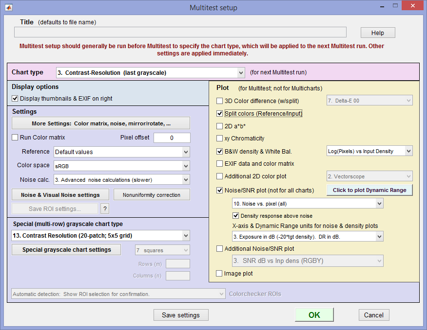
| 图表类型 | 选择图表类型。应用于下次运行。如果选择图表类型 3(最后灰度图)或 7(多行灰度阶梯图(非线性)),则应在下面的“特殊(多行)灰度图表类型”下拉菜单中选择具体的图表类型。 |
| 打开颜色/色调设置窗口,如下图所示。您可以选择颜色矩阵设置(详见颜色校正矩阵网页)、噪点设置、ISO感光度计算、mxn图表设置等,如下所述。 | |
| 运行颜色矩阵 | 如果选中,则计算并应用颜色校正矩阵(CCM)。 |
| 参考 | 参考文件。可以是标准格式,也可以是读取格式(通常从 CSV 或 CGATS L*a*b* 或密度文件读取)。具体格式会因图表类型而略有不同。 |
| 色彩空间 | 色彩空间 |
| 噪声计算。 | 噪声计算。选择 1. 无(非视觉)噪声计算(最快),2. 基本噪声计算(较慢),或 3. 高级噪声计算(较慢)。 |
| 噪声和视觉噪声设置 | 打开“噪点和视觉噪点”窗口,具体说明请参见“颜色/色调交互式/自动/eSFR ISO 噪点” 。您可以在此选择视觉噪点和其他设置。 |
| 非均匀性校正 | 允许您使用在相同条件下拍摄的单独平场图像来校正非均匀照明。打开“非均匀性校正”窗口,该窗口在灰度和彩色图表模块的“非均匀性校正”部分中进行了描述。 |
| 特殊(多行)灰度图表类型 | 仅当选择图表类型 3(最后灰度图)或 7(多行灰度阶梯图(非线性))时可见。用于选择合适的灰度图表类型。 |
| 特殊灰度图表设置 | 打开一个窗口,允许您选择线性灰度阶梯图的密度增量。 |
| 在右侧显示缩略图和 EXIF 信息。 | 在图表右侧显示整幅图像和裁剪区域的缩略图以及 EXIF 结果。示例如下所示。 |
| 绘图设置(右侧) | 选择输出数据。具体说明如下。 |
| 颜色校正矩阵 | CCM 计算的设置说明请参见“颜色校正矩阵”页面。 |
| 事件 Lux | 必须手动输入ISO感光度(曝光指数)计算所需的参数。光圈和曝光时间(秒)通常从EXIF数据中获取,但如果EXIF数据缺失,则可以手动输入。 |
| 噪音 | 设置说明请参见“颜色/色调/eSFR ISO 噪点”页面。 |
| 行、列 通用 MXN 图表 | 选择通用m x n (矩形)图表的行数和列数。选择此图表需要参考文件。 |
| 饱和度 | 输入图像的最大像素级别(对应于饱和度级别),用于对图像数据进行归一化以进行某些计算。 标准文件:255(或 65535...) :饱和度级别会根据图像数据的数据类型和容器大小自动设置。这是默认设置。图像文件假定具有标准位深度(例如,8 位、16 位或 32 位数据)和标准饱和度级别。例如,对于标准的 8 位图像数据,饱和度级别将设置为 255。对于 16 位图像,饱和度级别将设置为 65535,而对于 32 位图像,饱和度级别将设置为 4294967295。 ITU-R 建议 601 (BT. 601: 235) :饱和度级别设置为 235。 最大检测到的色块级别:饱和度级别设置为图像中色块区域检测到的最大值。如果图像数据的位深度不标准(例如,12 位数据存储在 16 位容器中),或者存在自定义饱和度级别,只要图像曝光足以使最亮的色块达到饱和状态,此功能就非常有用。 手动输入饱和度:饱和度级别设置为用户输入的值。如果图像数据的位深度不标准,或者存在自定义饱和度级别,则此功能非常有用。例如,对于存储在 16 位容器中的 12 位数据的图像,饱和度级别应输入 4095(2^12 - 1 = 4095)。 |
| 像素偏移 | 输入要从数据中减去的像素偏移量。像素偏移量并不罕见:它们会导致密度曲线过早趋于平缓。 |
| 非均匀性校正 | 允许您使用在相同条件下拍摄的单独平场图像来校正非均匀照明。打开“非均匀性校正”窗口,该窗口在灰度和彩色图表模块的“非均匀性校正”部分中进行了描述。 |
| 图像方向 | (适用于下次读取)选择标准图像方向、镜像(水平翻转)、镜像(垂直翻转)、旋转 180 度。 |
参考文件
大多数图表都允许使用“设置”区域中的“参考”下拉菜单输入参考文件。(IT8.7 图表必须使用参考文件。)可用设置取决于图表类型。通常,上一个参考文件会在下拉列表中显示。以下是可用参考源的概述。
| 您可以从“颜色/色调交互式”窗口获取当前参考数据,方法是按“文件”(左上角的下拉菜单),“复制 L*a*b* 参考到剪贴板”,或者按“文件”,“复制密度参考到剪贴板”。 |
| 图表 | 默认值 | 选项(来自文件的数据) |
| X-Rite ColorChecker (24 补丁) | X-Rite 、 BabelColor或 Danes Picta(一种几何形状相同但颜色不同的图表)的默认值 | L*a*b*、xyY D50 或 xyY D65 文件,CSV 格式。 |
| IT8.7 | 需要 IT8.7 格式的参考文件,该文件可从海图制造商处获得,通常可在其网站上找到。 | — |
| Rezchecker | 您可以使用ISA提供的标准默认参考数据或 NIST 可溯源测量数据。这些测量数据采用难以使用的 XLS/CGATS 文件格式。要使用这些数据,请在 Google 表格(可直接在 Gmail 中打开)或 Excel 中打开该文件。选择代表色块的 30 行和代表 LAB L、LAB A 和 LAB B 的 3 列,并将它们复制到剪贴板。然后将其粘贴到文本编辑器中并保存文件(文件扩展名为 txt 或 csv)。 带有光泽灰度色块(最大密度 = 2.42)的图表版本的参考数据已内置于“颜色/色调”模块中。带有哑光灰度色块(最大密度 = 1.485)的图表版本的参考文件可在此处下载。 | |
| X-Rite ColorChecker SG | X-Rite的默认值(L*a*b* D50);参见下方注释 | L*a*b*、xyY D50 或 xyY D65 文件,CSV 格式。 |
| 阶梯图(线性) | 密度步长为 0.1、0.15、0.20 或 0.30。仅对于UTT ,L* = 95 到 5,前 19 步以 -5 为步长,第 20 步以 1 为步长。(20 步 UTT)应选择。 | 您可以输入一个ASCII密度参考文件,其中每行包含一个密度值。 |
| 图像工程TE269 (36 个补丁) | 三个标准参考文件源自制造商网站上的数据: TE269A | TE269B | TE269C。Imatest 36色块图表提供单独测量的参考文件。 | 您可以在Imatest ROI 选项窗口中选择旧版 TE269 或新版 TE269V2。)注意:不建议使用 20 片 OECF 图表进行动态范围测量。 |
| 注意:一些默认参考值源自 L*a*b* D50 值,即在 D50 照明条件下采集的 L*a*b* 值。当色彩空间的参考色温不同时(sRGB 和 Adobe RGB 的参考色温均为 D65),系统会应用 Bradford 变换,导致 L*a*b* 值略有变化。如果您在不同的光源下拍摄图像,这通常不会造成显著影响:如果白平衡算法工作正常,它会将图像颜色转换为适合该色彩空间的相应值。 | ||
除 IT8.7 外,参考文件必须为 CSV(逗号分隔值)或 CGATS 格式。CSV 文件可在 Excel 中打开和编辑。颜色文件(L*a*b*、xyY D50 和 xyY D65)每行包含三个条目;密度文件每行包含一个条目。
以下是一个 L*a*b* 文件的示例。
格式为 CSV(逗号分隔变量)。
xyY 文件的格式相同。
添加空格仅为提高视觉清晰度(可读性)。
28.778, 14.179, -50.297
65.711、18.13、17.81
51.038, -28.631, -28.638
51.935, 49.986, -14.574
81.733、4.039、79.819
42.101、53.378、28.19
如果您有分光光度计,您可以使用测量测试图表色块中描述的技术创建自定义参考文件(CGATS 格式)。
测试图表的颜色参考包含图表中每个色块的 CIELAB(设备无关的 L*a*b*)值。它可以是
关于以下方面的色温问题经常出现:(1) 用于测量参考文件中色块的色温;(2) 用于根据色卡图像测量相机色彩准确度的色温;以及(有时会被忽略的)(3) 被测相机所使用的色彩空间中内置的色温。(所有可互换文件都与其关联的色彩空间相关联,无论是隐式的还是显式的。) 色块的测量使用已知色温的光源,通常为 5000K。色彩空间具有一个光源白点。sRGB (广泛使用的 Windows 互联网标准)的光源白点为 6500K,环境(观看环境)白点为 D50(约 5000K)。维基百科对此解释不多,但6500K 光源白点是该文件的主要属性。通常使用Bradford 变换将 5000K 的测量值转换为 6500K 色彩空间的光源白点。 一个常见的问题是:“使用与色温白点(通常为 6500K)不同的光源测量色温表时,是否需要特殊的参考文件?”这个问题很重要,因为Imatest测量(实际上几乎所有相机操作)都可以在各种色温下进行,从白炽灯的 2400K 到某些日光条件下的 10000K 以上。简而言之,答案是“不需要” 。 应使用标准参考文件。相机通常会通过算法对原始图像进行转换,该算法会估算光源色温,然后应用色彩校正矩阵 ( CCM ) 对图像进行白平衡和色彩校正。Imatest 也可以将 CCM 应用于未经校正的图像。 |
结果数据
1. 3D 色差(带分割)
在此图中,区域的高度代表选定的颜色差异,在本例中为 ΔE* ab (即 Delta-E)。色块平台的顶部以双色显示,左上角为参考颜色,右下角为实际输入颜色。此图可用于比较测量颜色与感知颜色差异。(它们可能与理论声称的匹配度不完全一致。)
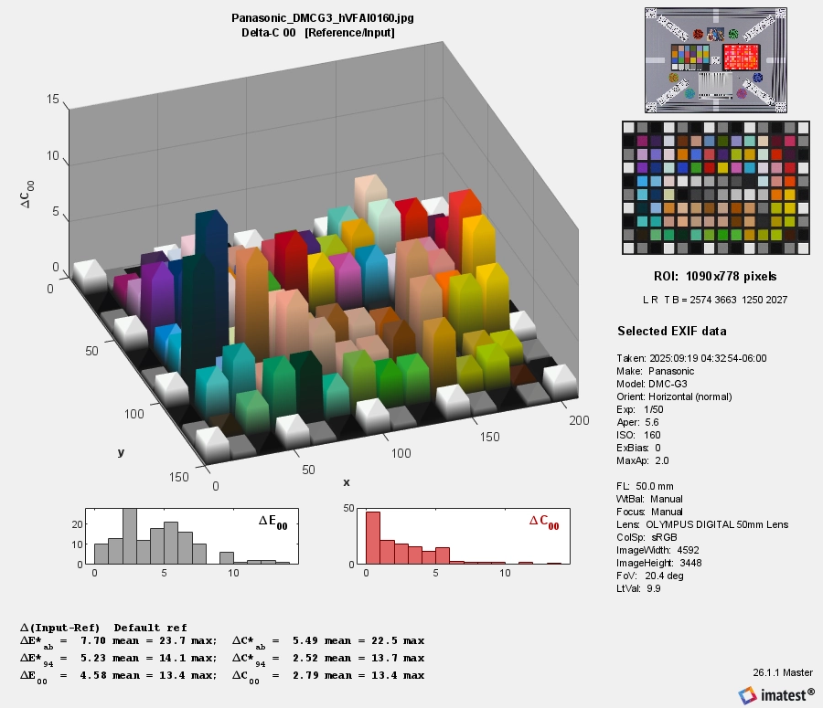
此图表右侧会显示缩略图和 EXIF 数据(在“颜色/色调自动设置”窗口中勾选复选框即可设置)。其他图表将不显示这些结果,即未勾选该复选框(这样可以节省空间)。
2. 分割颜色(参考/输入)图分割颜色图显示左上角的参考(理想)颜色和右下角的输入颜色。 如果已计算颜色校正矩阵(如果已选中复选框),则此图以及 3D 颜色差异图(上图)将在左上角显示参考颜色,在右上角显示输入颜色,在底部显示校正后的颜色。 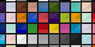 | 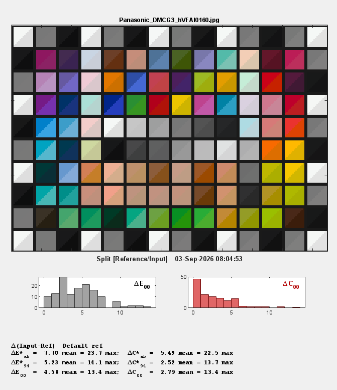 | |
3. 二维 a*b* 图显示 L*a*b* 色彩空间的 a*b* 平面。色度差异(非常)近似于参考值和相机值之间的距离。(此差异为 ΔC <sub>ab</sub> 。更复杂的 ΔC<sub> 94</sub>和 ΔC<sub> 00 </sub> (CIEDE 2000) 方程(此处有描述)更为精确。) 如果已计算出颜色校正矩阵,则会显示校正后的值。 | 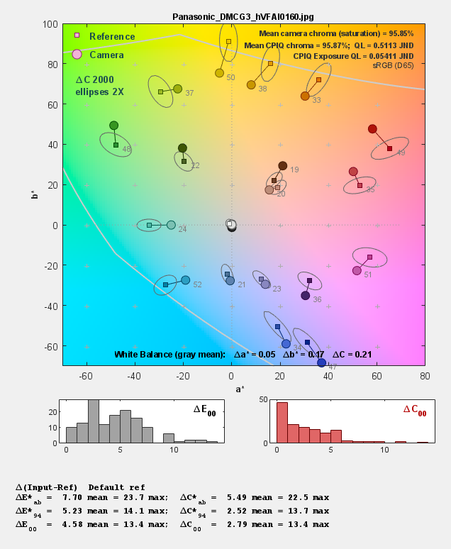 | |
4. XY色度这张图虽然很常见,但与上面的a*b*图相比,在视觉上不够均匀。绿色在这张图中占据的面积过大。 如果已计算出颜色校正矩阵,则会显示校正后的值。 | 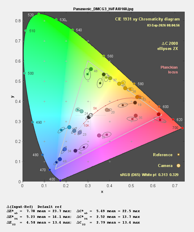 | |
5. 黑白密度和白平衡上图显示 Log(像素级别/255)(最大值为 1)与输入密度(-log 10 (曝光))的关系,即使用密度单位。 下图展示了几种不同色块密度下的ΔC值。参见颜色检查附录。 如果已计算出颜色校正矩阵,则会显示校正后的值。 | 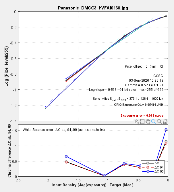 | |
6. EXIF 数据和颜色矩阵该图显示了选定的 EXIF 数据和颜色矩阵校正结果,包括
| 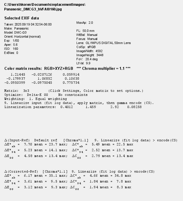 | |
7. 附加二维彩色图此处显示矢量示波器界面。您可以在此处选择几个图表之一:
这些显示方式在“使用颜色/色调 - 显示和选项”中有详细说明。 | 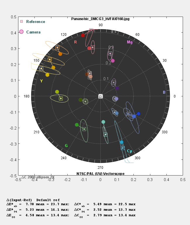 | |
噪声/信噪比分析(并非所有图表都适用)噪声/信噪比分析仅适用于图像块足够大、能够提供良好噪声统计数据的图表。噪声分析包括标准像素噪声、色度噪声、场景参考噪声、传感器(原始)噪声和 ISO-15739 视觉噪声。信噪比 (SNR) 可以以比值或分贝 (dB) 的形式显示。 本页所示的 ColorChecker SG 色块太小,但幸运的是,Imaging-Resource 图像在 SG 的左侧有一个标准的 24 色块 ColorChecker,我们对其进行了分析,从而得到了右侧所示的结果。 噪声分析在“颜色/色调”和“eSFR ISO 噪声”部分有详细描述。ISO 15739 视觉噪声已添加到Imatest 4.0中。 可供选择的选项如下。
| 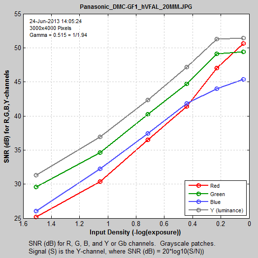 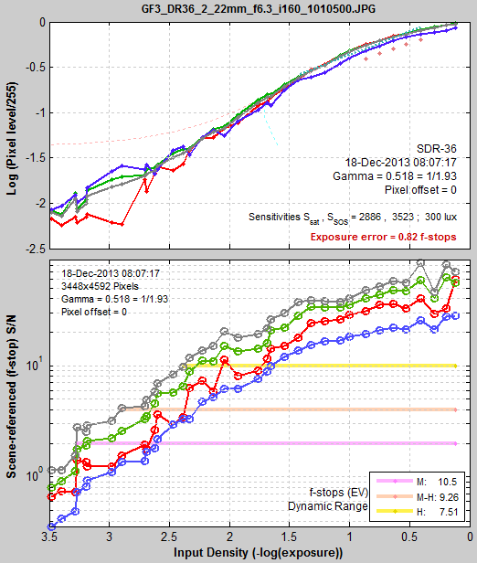 |
 3D色彩差异细节,