Measurement of vignetting and sensor nonuniformity
This page covers running a flat-field analysis and the settings that control it, for both the Interactive and the Auto interfaces. Use the selector to switch between them: the choice applies to the whole page. The measurements themselves are described in Flat Field results.
Flatfield-Interactive measures image nonuniformity, which can be caused by the lens, the sensor, and the lighting— the same parameters measured by Flatfield— in an interactive interface that can be updated in near-realtime. It can also photo response nonuniformity (PRNU) derived from the EMVA 1288 standard, ISO 18844 flare (veiling glare), and more.
Flatfield-Interactive can display pixel and color shading contour plots, pixel level histograms, hot and dead pixels, grid and grid contour plots, and much more. The table below contains a complete list of displays. Many of the features are also described in Using Flatfield and Using Flatfield Part 2.
Image preparation | Running | Controls | Settings window | Results
Luminance contour plot | f-stop contour plot | Grid contour map | CSV & JSON output | Saving results
 Instructions
To prepare an image for Flat Field,
- If possible, set your camera or lens to manual focus and focus it at infinity (the worst case for light falloff).
- Photograph an evenly illuminated uniform subject.
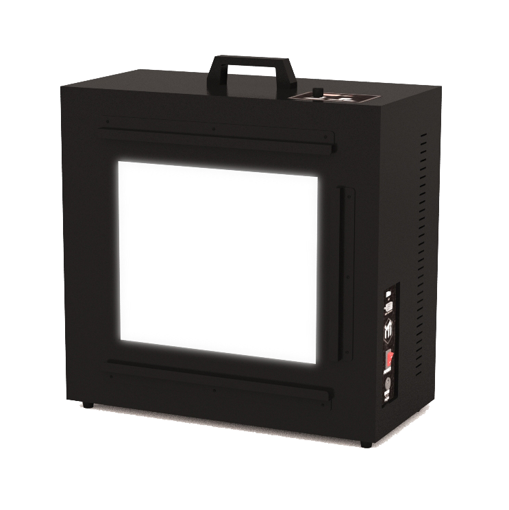
- To obtain even illumination we recommend an Imatest LED LIghtbox. There are several models. Features excellent illumination uniformity (90-95%), dimming over a range of 30 lux to 10,000 lux in standard models (with options as low as 1 lux and up to 100,000 lux), selectable color temperatures (3100K, 4100K, 5100K, 5500K, 6500K, NIR 850nm, NIR 940nm), and can be used with Imatest Dynamic Range and other transmissive charts. Imatest lightboxes are compared here.
|
The following techniques— an LCD monitor (most have flicker or have a fine structure) or a flat reflected sheet (hard to illuminate evenly) are no longer recommended. We've kept the instructions only for reference. 
|
- The subject does not need to be in focus (you don't even need a lens to measure sensor uniformity); the goal is to measure lens light falloff and/or sensor uniformity, not features of the subject. For typical measurements, set exposure compensation to overexpose by about one f-stop. (You may, however, use any exposure you choose.)
- Save the image as a RAW file or maximum quality JPEG.
Image preparation
- If possible, set your camera or lens to manual focus and focus it at infinity (for minimum light falloff).
-
Photograph an evenly illuminated uniform ("flat field") subject.
To obtain even illumination
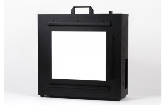
We recommend an Imatest LED LIghtbox or Light Panel. The Lightbox features excellent illumination uniformity (97%), dimming over a range of 300:1, selectable color temperature (typically 3100 and 5100K), and can be used with Imatest Dynamic Range and other transmissive charts. Lightboxes are compared here.
The most even illumination can be obtained with an integrating sphere (not sold by Imatest), but the Imatest lightbox and panel should be more than sufficient for most applications because they are typically very close to camera.
|
- The subject does not need to be in focus (you don't even need a lens to measure sensor uniformity); the goal is to measure lens light falloff and/or sensor uniformity, not features of the subject. For typical measurements, set exposure compensation to overexpose by about one f-stop. (You may, however, use any exposure you choose.)
- Save the image as a RAW file or maximum quality JPEG.
Running the analysis
Running Flatfield Analysis in the New Main Window:
- Select your Image, then click Next to Select Analysis options.
- In Analysis Options screen - in Targets, open the "Uniformity/Blemish" Category, and select Flat Field.
- There is a radio button at the bottom of the analysis card that allows you to select the Interactive (or Automatic) mode. Select the desired mode.
- Click Analyze - the ROI option screen will appear, (choose the desired ROI and click yes), then the Flatfield Interactive results screen will be displayed.
- There are buttons on the bottom of the page to change Settings for Uniformity and Blemish. (The settings are described in detail below.)
- Use the dropdown menu on bottom left of the results screen, to choose a different output display.
- Results can be saved using the Save screen or Save Data buttons. When done, click Exit to return to Main Window.
Running Flatfield Analysis from the Classic UI:
- Start Imatest, choose Classic UI from the Main Menu. When the Classic interface appears, click on .
- A dialog box will open and that prompt you to select input image file(s).
More About Files:
- Very large files (height x width x colors over 40 MB) sometimes caused memory overflow problems with (older) 32-bit systems. Files over 40 or 80 MB can be automatically reduced 1/2x linearly (using 1/4 the memory). In Settings, make the appropriate setting in LARGE FILES (Uniformity, Distortion). This should be unnecessary with recent versions of Imatest.
- Open the image file.
Multiple file selection Several files can be selected in Imatest Master using standard Windows techniques (shift-click or control-click). Depending on your response to the multi-image dialog box you can combine (average) several files or run them sequentially (batch mode). Combined (averaged) files are useful for measuring fixed-pattern noise (at least 8 identical images captured at low ISO speed are recommended). The combined file can be saved. Its name will be the same as the first selected file with _comb_n appended, where n is the number of files combined. Batch mode allows several files to be analyzed in sequence. There are three requirements. The files should (1) be in the same folder, (2) have the same pixel size, and (3) be framed identically. The input dialog box for the first run is the same as for standard non-batch runs. Additional runs use the same settings. Since no user input is required they can run extremely fast. Caution: Imatest can slow dramatically on most computers when more than about twenty figures are open. For this reason we recommend checking the Close figures after save checkbox, and saving the results. This allows a large number of image files to be run in batch mode without danger of bogging down the computer. Three cropping (ROI selection) options are available in Settings, under ROI Options. These include
1. Enable "Crop pixels near borders" in Settings box. (Don't ask to crop.) 2. Select crop (ROI) by dragging cursor. Ask to repeat crop for same sized image [default]. 3. Select crop (ROI)by dragging cursor. Do not ask to repeat crop. 4. Automatically select crop for image surrounded by a dark boundary. The second option (Select crop by dragging cursor. Ask to repeat crop for same sized image), which is similar to the ROI selection in SFR, is typically preferred

Input dialog box in Imatest Master
The settings described below are available in Imatest Studio, i.e., they appear in all Imatest versions. Additional settings are described in Using Flat Field, Part 2.
- Title Defaults to the file name. You can change it if you wish.
- Contour plots (Plot area; on by default). Often set to Display pixel and f-stop contours (two plots), but may be turned off or set to display only. Available settings are
| No contour plots |
| Display pixel and f-stop contours |
| Display pixel contours only |
| Display f-stop contours only |
- Contour plot display options Eight display options are available. 3D plots are not generally recommended because they can be slow. Normalized refers to the first (level) plot only (not to the displayed numeric results).
| Contours superposed on image (not normalized) |
| Contours superposed on image (normalized to 1) |
| Pseudocolor with colorbar (not normalized) |
| Pseudocolor with colorbar (normalized to 1) |
| 3D pseudocolor w/colorbar (not normalized) |
| 3D pseudocolor w/colorbar (normalized to 1) |
| 3D pseudocolor shaded w/colorbar (not normalized) |
| 3D pseudocolor shaded w/colorbar (normalized to 1) |
- Scaling options
| Auto or manual scaling: Set with Scaling. | Scaling set by button. |
| Scaling: 0 - 1 or 255: -4 - 0 f-stops | Fixed scaling: 0 - 1 or 255 for Luminance pixel plot; -4 - 0 f-stops for f-stop plot. |
| Scaling (min - max) | Fully automatic scaling. |
-
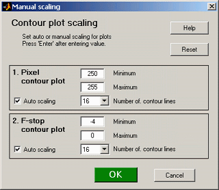
Manual scaling for contour plots
Contour plot scaling Scale to 1 or Scale to 255
sets the scaling for the pixel level (the first) contour plot.
- : Opens a dialog box that lets you select manual or automatic scaling for the two contour plots. Minimum and Maximum set the scale when Auto scaling is unchecked.
- Extra smoothing applies extra smoothing to the contour plots, making them less susceptible to variations from noise (and faster to plot). Strongly recommended. Uncheck this box only for compatibility with older results.
- Speedup When checked, several results (those that require significant calculation time) are not calculated (and hence not saved in the CSV output file) if the corresponding plot is not selected. This can save significant time in production environments. If you need to use Speedup, you should run Flat Field with and without Speedup checked and examine the CSV output file to see if it contains the results you require.
- Corner and side regions (default 32x32 pixels) allows you to select the areas at the corners and sides of the images to be analyzed. These affect the numeric readouts below the plots (example: Corners: worst = ...). Choices include 10x10 pixels, 32x32 pixels, 1% (min. 10x10), 2% (min. 10x10), 5%, and 10%.
- Location Location of corner and side regions in units of image height (0, 1%, 2%, 5%, 10%, 15%, 20%). 0% was always implied prior to Imatest 3.8 (corner and side regions always abutted the image boundaries).
- Gamma (Settings area). The default value of gamma, 0.5, is typical for digital cameras. Gamma affects the second figure (the light falloff measured in f-stops); it has no effect on the first figure. Gamma can be measured by Stepchart using any one of several widely-available step charts. (Reflection charts are easiest to use but transmission charts can also be used to measure dynamic range.) Some issues in calculating gamma are discussed below the second figure.
- Crop pixels near borders (L, R, T, B) (Settings area). Available only if Don't ask to crop. (Use Crop ... borders settings in LF input dialog box.) is selected in Settings. If checked, the image is cropped by the number of pixels indicated near the left, right, top, and bottom borders.
- Crop pixels near borders (L, R, T, B) (This feature is normally disabled.) Enabled only if Don't ask to crop. (Use Crop ... borders settings in LF input dialog box.) is selected in the Options I. If checked, the image is cropped by the number of pixels indicated near the left, right, top, and bottom borders.
Two methods of region selection
The region to be analyzed (ROI) is normally set in the coarse and fine region adjust windows, where the ROI is defined relative to the upper-left corner, not to each of the edges. So if you want a constant margin for several images (for example, you want the ROI boundaries to be 4 pixels from the borders), ROI must be set individually for each image size.
Blemish Detect offers an alternative method of specifying the ROI relative to the image boundaries: crop_borders, which is set with Crop pixels near borders near the bottom of the Uniformity (or Blemish) window when (Use Crop ... borders settings in LF input dialog box.) is selected in and the Crop pixels... box is checked. Otherwise, crop_borders is ignored and the standard ROI selection is used.
The following options are discussed in detail in Flat Field instructions: Imatest Master .
- Channel (Settings area) You can choose between Red, Blue, Green, and Y (luminance) channel
- Hot and dead pixels (Settings area) By checking the appropriate boxes you can display hot pixels (redx) and/or dead pixels (blue •). Hot pixels are defined in an absolute sense: stuck at or near the sensor's maximum value (255 in 8-bit files) and dead pixels are stuck at or near 0, or in a relative sense. You can choose between hot/dead pixel detection in any channel, all channels or the selected channel.
 Because signal processing— especially JPEG compression— can cause these values to shift, you can use the sliders to set the detection threshold between 6-255 for hot pixels and 0-249 pixels for dead pixels. (The extreme values are for measurements made on white or black fields.) Clicking on or at the ends of the sliders adjusts the threshold by 1. The default values are 252 and 4, respectively. Settings are saved between runs. JPEG files must be saved at the highest quality level for this feature to work; isolated hot and dead pixels tend to be smudged at lower quality levels. Details are described in Flat Field part 2.
- (Plot area)
- Color shading displays color nonuniformity. Several options are available.
- Color uniformity profiles displays R, G, and B values (or ratios— several options available) along the diagonals and horizontal and vertical center lines.
- Display Histogram displays histograms of R, G, and B channels.
- Fine detail plot displays a detailed figure of noise and sensor uniformity with an option for spot detection.. The calculation can be slow and uses lots of memory. To a large extent it has been replaced by Blemish Detect. Details in Flat Field: Imatest Master.
Flatfield Interactive - file selection:
Very large files (height x width x colors over 40 MB) sometimes caused memory overflow problems on older 32-bit systems. Files over 40 or 80 MB can be automatically reduced 1/2x linearly (using 1/4 the memory) in Settings, by making the appropriate setting in LARGE FILES (Flatfield, Blemish...).
| 1. Use "Enable Crop pixels near border" in Settings box (Don't ask to crop.) |
| 2. Select crop (ROI) by dragging cursor. Ask to repeat crop for same sized image [default]. |
| 3. Select crop by dragging cursor. Do not ask to repeat crop. |
| 4. Automatically select crop for image surrounded by a dark boundary. |
After the input file has been read, the Flatfield-Interactive window, showing the most recently displayed results, is displayed.
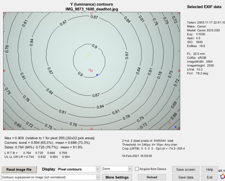
(identical to the first figure of Flatfield)
Results are displayed using the previous settings (saved in imatest-v2.ini), in this case the pixel contour plot with unnormalized contours superposed on the image.
Flatfield controls
- reads an image, then performs calculations and displays results.
- Display dropdown menu selects the results to display. Selections are shown in the Table, below.
- Primary display settings (below Display) lets you select the most important settings for the selected display, for example how to normalize the results, whether to display a pseudocolor plot, etc. Additional settings are available by pressing , immediately to the right.
- opens the Flatfield Uniformity Settings dialog box, shown below. This contains advanced settings not shown in the Primary display settings dropdown menu.
- The Blemish button opens the Blemish Detect settings dialog box.
-
Zoom/Rotate 3D/Data Cursor
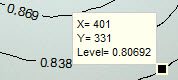
selects the action when you click on the image. Zoom zooms in on the image. It zooms out when you shift-click or double-click. Rotate 3D is used to rotate 3D images (2D images are zoomed). Data Cursor opens a tiny window called a Datatip that displays values of the image or curve. Right-click on the Datatip to remove it or access additional options. - checkbox may be removed because Settings, Device manager is better for setting up direct acquisition.
- reloads the image. Most valuable for Image Acquisition, which allows images to be read directly from devices like USB cameras or manufacturer's evaluation boards.
- Saves and optionally displays the Flatfield window.
- Saves results in CSV and/or XML files. Opens the Save dialog box.
- opens this web page. (Others are available in the Help dropdown window on the top toolbar.)
- exits the Flatfield window.
Flatfield-Interactive settings window
The settings window opens when you answer Yes (not Express mode) when reading an image or when you press the Uniformity button at the bottom of the Flatfield Interactive screen. It is similar to the Flatfield settings window, but some display selections are missing because they're made in the Flatfield-Interactive Display dropdown menu.
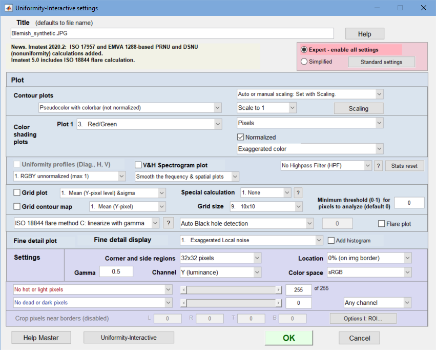
- Title Defaults to the file name. You can change it if you wish.
- Expert/Simplified modes Simplified mode grays out advanced selections that may not be needed by beginners.
- selects commonly-used settings: good choices for beginners.
Plot area
Most of the settings in this area apply to displays that are selected in the Flatfield-Interactive window. For this reason, Some display selections used in Flatfield are missing (or disabled). (And a few should probably be disabled.) Some of the settings listed below are duplicated in the Primary display settings dropdown menu of the Flatfield-Interactive window.
- Contour plot display options Eight display options are available. 3D plots are available. Normalized refers to the Pixel contour display only.
| Contours superposed on image (not normalized) |
| Contours superposed on image (normalized to 1) |
| Pseudocolor with colorbar (not normalized) |
| Pseudocolor with colorbar (normalized to 1) |
| 3D pseudocolor w/colorbar (not normalized) |
| 3D pseudocolor w/colorbar (normalized to 1) |
| 3D pseudocolor shaded w/colorbar (not normalized) |
| 3D pseudocolor shaded w/colorbar (normalized to 1) |
| Manual scaling for contour plots |
- Color shading (Plot 1): Select Red/Blue, Red/Green, Green/Blue, or any of several variants of ΔE and ΔC (76 (i.e., plain), 94, and 2000).
- Display type: Exaggerated color, Pseudocolor, and 3D options.
- Pixels (gamma-encoded), Intensity (linear— using gamma), and f-stop difference.
- (Dropdown menu below Uniformity profiles) Choose between several different normalizations or R, G, B, and Y, R/G and B/G, or Delta-L*, a*, b*, and C*.
- (Dropdown menu below V&H Spectrogram plot) Select frequency & spatial plot smoothing.
- Highpass filter (HPF) dropdown: Turn on box HPF for EMVA 1288 calculations. Used for histograms.
- (Dropdown menu to right of Grid plot) Select parameters to display: mean & sigma, Delta-C & Delta-E, etc.
- (Dropdown menu to right of Grid contour map) Select a single parameter to display (value and contour). Settings listed below.
- Special calculation: None, CPIQ, or ISO 17957.
- Grid size for Grid plot and contour map. From single region to 32×18. 10×10 is typical.
Fine detail display Choose between exaggerated local noise with or without contour lines, pseudocolor contours, spot detection (which includes nonlinear processing), or several 3D plots.
Settings area
- Gamma Gamma is the average slope of the log pixel level vs. log exposure curve, taken from a specified maximum value through dark gray values. It only affects the f-stop contour plot and ISO 18844 flare measurements; it has no effect on the other measurements. The default value (0.5) is typical for digital cameras. Gamma is measured by Color/Tone Interactive or Auto using any one of several widely-available grayscale step charts, or by legacy modules Stepchart or Colorcheck. Some issues in calculating gamma are discussed next to f-stop contour plot.
- Corner and side regions (default 32x32 pixels) allows you to select the areas at the corners and sides of the images to be analyzed. These affect the numeric readouts below the plots (example: Corners: worst = ...). Choices include 10x10 pixels, 32x32 pixels, 1% (min. 10x10), 2% (min. 10x10), 5%, and 10%.
- Crop pixels near borders (L, R, T, B) (Settings area). Available only if Don't ask to crop. (Use Crop ... borders settings in LF input dialog box.) is selected in Settings. If checked, the image is cropped by the number of pixels indicated near the left, right, top, and bottom borders.
- Color space affects Color shading ΔE and ΔC measurements in Color Shading, Grid, and Grid Contour plots.
The following options are not available in Imatest Studio. They are discussed in detail in Using Flatfield Part 2.
- Channel You can choose between Red, Blue, Green, and Y (luminance) channel
- Hot and dead pixels By checking the appropriate boxes you can display hot pixels (red ¤) and/or dead pixels (blue •). Hot pixels are stuck at or near the sensor's maximum value (255 in 8-bit files) and dead pixels are stuck at or near 0. You can choose between hot/dhead pixel detection in any channel, all channels or the selected channel.

Because signal processing— especially JPEG compression— can cause defect pixel levels to shift, you can use the sliders to set the detection threshold between 6-255 for hot pixels and 0-249 pixels for dead pixels. (The extreme values are for measurements made on white or black fields.) Clicking on or at the ends of the sliders adjusts the threshold by 1. The default values are 252 and 4, respectively. JPEG files must be saved at the highest quality level for this feature to work; isolated hot and dead pixels tend to be smudged at lower quality levels. Details are described in Using Uniformity Part 2.
Dropdown menus
There are four dropdown menus, located just below the top of the Flatfield Interactive window: File, Settings, INI File Settings, Help.
File contains several file-related functions
- Read image file
- Save image to file
- Save temporal noise image. Only applies when temporal noise is calculated — when signal averaging is applied and Calculate image^2 while averaging is checked
- Save pseudo-raw/remosaiced image — Save the image as an undemosiaced (Bayer raw image).
- Save screen — displays screen and optionally saves it (most of the time we don't save the screen)
- Open image file folder
- Open recent save folder
- Preview JSON results
- View all EXIF data
- Image statistics/viewer
- Close
Settings
- Small, Normal, Large, X-Large fonts
- Reset screen — resets screen to original size and position (above the Main Window)
- Image from file
- Device manager — Opens the Device manager for selecting an image acquisition device, adjusting the settings, and previewing the image.
- Image from device > Lets you select a device for acquiring an image. Not recommended. Device manager is more reliable.
- Signal averaging > Lets you average up to 128 directly-acquired images for reducing noise and for separating temporal and spatial noise in EMVA-1288-based nonFlatfield calculations and for calculating noise images.
- Calculate image^2 while averaging. Required for separating spatial and temporal noise
Input settings
The following settings are available in all Imatest versions:
-
- Title Defaults to the file name. You can change it if you wish.
- Display Uniformity contour plots (Plot area; on by default).
Turns the main light falloff contour plots off or on. Normally on (checked), but may be turned off by Imatest Master users interested in other results, such as hot/dead pixels and color shading. Four display options are available. Normalized refers to the first (level) plot only.
Examples on Using Flat Field, Part 1.
| Contours superposed on image (not normalized) |
| Contours superposed on image (normalized to 1) |
| Pseudocolor with colorbar (not normalized) |
| Pseudocolor with colorbar (normalized to 1) |
- Speedup When checked, several results (those that require significant calculation time) are not calculated (and hence not saved in the CSV output file) if the corresponding plot is not selected. This can save significant time in production environments. If you need to use Speedup, you should run Flat Field with and without Speedup checked and examine the CSV output file to see if it contains the results you require.
- Gamma The default value of gamma, 0.5, is typical for digital cameras. Gamma affects only the second figure (the light falloff measured in f-stops); it has no effect on the first figure. Gamma can be measured by Stepchart using any one of several widely-available step charts. (Reflection charts are easiest to use but transmission charts can also be used to measure dynamic range.) Some issues in calculating gamma are discussed below the second figure.
- Corner and side regions (default 32x32 pixels) allows you to select the areas at the corners and sides of the images to be analyzed. Choices include 10x10 pixels, 32x32 pixels, 1% (min. 10x10), 2% (min. 10x10), 5%, and 10%. These regions can be used as the reference for the Color shading ΔE and ΔC calculations.
- Crop pixels near borders (L, R, T, B) (Settings area). If checked, the image is cropped by the number of pixels indicated near the left, right, top, and bottom borders. Several cropping (ROI selection) options are available in Settings. These incluce
Don't ask to crop. (Use settings in LF input dialog box.) Select crop by dragging cursor. Ask to repeat crop for same sized image. Select crop by dragging cursor. Do not ask to repeat crop. Although the first option (Don't ask to crop...) was the default prior to Imatest 2.3.12, the second option (Select crop by dragging cursor. Ask to repeat crop for same sized image), which is similar to the ROI selection in SFR, may be preferred.
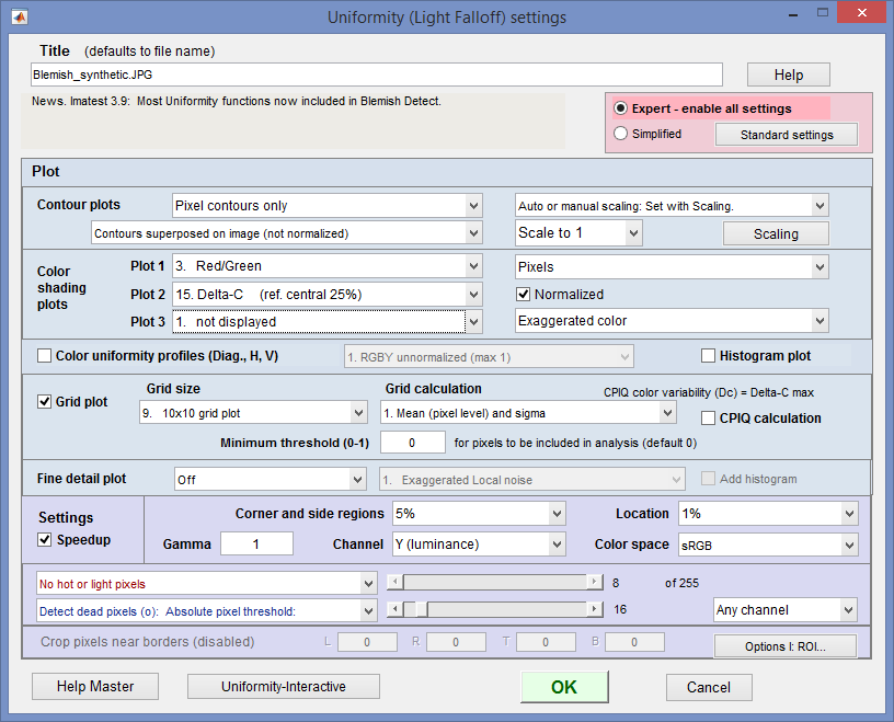
Uniformity settings window (for Imatest Master).
The following options are available in Imatest Master and IT:
- Color shading (nonuniformity) Display the color nonuniformity, i.e., the quotient of or difference between two of the three (R, G, B) channels or one of the L*a*b* color difference metrics (ΔE = sqrt(ΔL*2 + Δa*2 + Δb*2 ), ΔC = sqrt(Δa*2 + Δb*2 ), ΔE94, ΔC94, ΔE00, ΔC00 ), referred to the center of the image (either the central region, with size specified in the Corner and side regions box or the central 25% by area). Color shading often results from the angle at which light strikes the sensor. It tends to be worst in sensors with tiny pixels. Several options are available. [Note: the center of the image is used for the reference for calculating ΔC and ΔE in the Color shading plots, but for the grid plot, which implements the CPIQ Phase 2 specification, the mean of the entire image is used as the reference for calculating ΔC and ΔE.]
- Color shading Select not displayed (turns off plot), Red/Blue, Red/Green, Green/Blue, or ΔE or ΔC (various flavors & reference regions). Red/Blue (the extremes of the spectrum) is the most popular choice for displaying shading. for (plot units). To the right of the Color shading box. Select Pixels (gamma-encoded), Intensity (linear), or f-stop difference. Grayed out if ΔE or ΔC metrics are selected.
Pixels Displays the ratio of the the pixel values for the selected channels. If Normalized is checked, the plot is normalized to 1.0 (maximum). Intensity (linear) Removes the gamma encoding of the image file using the value of Gamma entered and displays the ratio of the intensities for the selected channels. If Normalized is checked, the plot is normalized to 1.0 (maximum). F-stop Displays the f-stop difference between the selected channels. If Normalized is checked, the plot is normalized to 0 (maximum). - Display Select the display type. Four choices.
Examples are shown below
Exaggerated color 2D. Increases the color saturation to increase the visibility of color nonuniformities. Pseudocolor 2D 3D Pseudocolor, shaded, auto-scaled. Shading emphasizes contour shapes. 3D Pseudocolor, auto-scaled. - Normalized (Checkbox) If checked (the default), the shading plot is normalized to a maximum of 1 for quotient displays (Red/Green, etc.) Affects only the plot, not the numeric values beneath the plot. The unnormalized maximum and minimum and other values are displayed beneath the plot.
- Extra smoothing This increases the smoothing of the contour and shading plots. Checked by default and strongly recommended. When unchecked the contour and color shading plots are much bumpier, more susceptible to noise, and slower. This checkbox may be removed in a future version.
- Color shading Select not displayed (turns off plot), Red/Blue, Red/Green, Green/Blue, or ΔE or ΔC (various flavors & reference regions). Red/Blue (the extremes of the spectrum) is the most popular choice for displaying shading. for (plot units). To the right of the Color shading box. Select Pixels (gamma-encoded), Intensity (linear), or f-stop difference. Grayed out if ΔE or ΔC metrics are selected.
- Color uniformity profiles Shows pixel levels along diagonal, vertical, and horizontal lines. The specific display is selected in the dropdown menu on the right. Described below.
- Grid plot Display a grid of results. You can select the grid (m x n) and two parameters to be displayed at each grid location.
- Grid size: single region, 3x3 through 10x10, 20x15, 24x16, 32x18, 15x15,16x16, 20x20, 25x25, 27x27 (not in this exact order).
- Grid calculation:
- Mean (pixel level) and sigma,
- Color differences Delta-C and Delta-E, Delta-C 94 and Delta-E 94, Delta-C 00 and Delta-E 00,all calculated relative to the mean for the entire image. Note: The CPIQ color variability metric (D) is the maximum Delta-C in the grid plot. It is shown below the plot when Delta-C and Delta-E are selected.
- Mean (pxl) & Delta Color Temp K,
- R/G and B/G pixel ratios,
 CIELAB a* and b*,
- Mean (pixel level) and SNR (s/n), Mean (pixel level) and SNR (dB).
- Minimum threshold (0-1) (default = 0). A minimum threshold for pixels to be included in grid plot analysis. Useful for automatically excluding dark areas in images like the one on the right.
We can add more grid plot measurements on request.
- Histogram plot Useful in diagnosing stuck (hot and dead) pixels. Described below.
- Fine detail plot Display a detailed image of noise and sensor nonuniformity (examples below). Slow variations in image density— vignetting (low spatial frequencies) — are removed so that only short to medium range variations— sensor noise, dust spots, etc.— remain. The calculation can be slow and uses lotsof memory because Matlab calculations are performed in double precision mathematics, which requires 24 bytes per color pixel (8 bytes per channel).
Exaggerated local noise (standard) Local noise with added contours Pseudocolor contours with colorbar Spot detection w / threshold (pseudocolor) (Several additional 3D displays) Several display options are available. The first displays noise exaggerated by a factor of 10. The second superposes contour plots (from a smoothed version of the image) on the noisy image. The third produces a pseudocolor image of local nonuniformities (also smoothed) with a color bar (legend) on the right. The fourth emphasizes dark spots, usually caused by dust. A histogram can also be added beneath the fine detail plot.
- Channel You can choose between Red, Blue, Green, or Y (luminance) channels. Color space Used for converting from RGB color space where L*a*b* color difference metrics are displayed.
- Hot and dead pixels By checking the appropriate boxes you can display hot or light pixels (red x) and/or dead or dark pixels (blue •). The definition depends on whether Absolute pixel threshold or Relative % threshold is selected:
Display hot or dead pixels (o): Absolute pixel threshold Hot pixels are stuck at the sensor's maximum value (255 in 8-bit files) and dead pixels are stuck at 0. Because signal processing— especially JPEG compression— often causes these values to shift, you can use the sliders to set the detection threshold between 6-255 for hot pixels and 0-249 pixels for dead pixels. (The extreme values are for measurements made on white or black fields.) Clicking on or at the ends of the sliders adjusts the threshold by 1. The default values are 252 and 4, respectively. Display light or dark pixels (o): Relative % threshold Light pixels are more than the relative % threshold above the mean of the 8 neighbors; Dark pixels are more than the relative % threshold below the mean of the 8 neighbors. Clusters (in Imatest 4.0+) are defined as groups of two or more adjacent pixels. JPEG files should be saved at the highest quality level for this feature to work well; isolated hot and dead pixels tend to be smudged at lower quality levels. Details of hot and dead pixels are presented below. You can choose whether to count a pixel as hot or dead (light or dark) if the criteria are met by any color channel (the default), all channels, or the selected channel.
Saving results
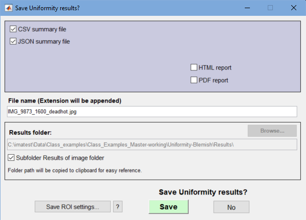 When you press the dialog box shown on the right is opened. It allows you to select which results to save (CSV and/or JSON files) where to save it. The default is subdirectory Results in the data file directory. You can change to another directory the results. CSV and JSON data are saved in files whose names consist of a root file name with a suffix for plot type and channel (R, G, B, or Y) and extension.
Example: IMG_9875_ISO1600_RGB_f-stop_ctrG.png. The root file name defaults to the image file name, but can be changed using the Results root file name box. Be sure to press enter. After you click on or , the Main Window reappears.
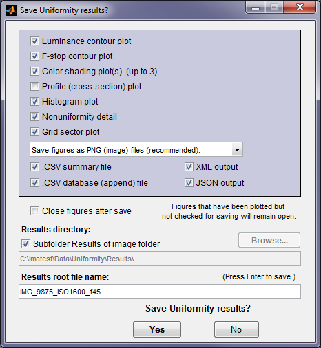 At the end of the run, a dialog box for saving results appears. It allows you to select figures to save and choose where to save them. The default is subdirectory Results of the image folder. You can change to another existing directory by unchecking the Subfolder Results of image folder check box. The selections are saved between runs.
You can examine the output figures before you check or uncheck the boxes. Figures, CSV, XML, and JSON results are saved in files whose names consist of a root file name with a suffix for plot type and channel (R, G, B, or Y) and extension. Example: IMG_9875_ISO1600_RGB_f-stop_ctrG.png. The root file name defaults to the image file name, but can be changed using the Results root file name box. Be sure to press enter. For batch runs, checking Close figures after save is recommended for preventing a buildup of figures (which slows down most systems). After you click on or , the Main Window reappears.
Figures can be saved as either PNG files (a standard losslessly-compressed image file format) or as Matlab FIG files, which can be opened with in the Utility menu. Fig files can be manipulated (zoomed and rotated), but they tend to require much more storage than PNG files, and are therefore not recommended.
The CSV and XML files contain EXIF data, which is image file metadata that contains important camera, lens, and exposure settings. By default, Imatest uses a small program, jhead.exe, which works only with JPEG files, to read EXIF data. To read detailed EXIF data from all image file formats, we recommend downloading, installing, and selecting Phil Harvey's ExifTool, as described here.