The plots and files a flat-field analysis produces. Where the Interactive and Auto interfaces present a result differently, both are shown: use the selector to switch. Running the analysis is covered in Running flat-field analysis.
Some results plots are described below on this page, but several are described on other pages, including Using Flatfield Part II, ISO 18844 Flare (Veiling glare), and Uniformity Statistics based on EMVA 1288 .
| Display (with link | Description |
| Original image | Original image, displayed uncropped. Several display settings are available: single channel, lighten, color boost, etc. |
| Luminance contours | Standard luminance (Y) channel contour plot. Several types of display are available: 2D, 3D, image or pseudocolor background. |
| F-stop contours | f-stop contour plot, converted from pixel levels using gamma setting. |
| Color shading | 2D or 3D contour plot of pixel ratios or ΔC and ΔE (ab, 94, or 2000) |
| Uniformity (Color) profiles | H, V, and diagonal profiles. |
| Histograms | R, G, B histograms of the image crop |
| Noise Fine detail | Somewhat interesting display of noise detail, but largely replaced by Blemish Detect. |
| Grid plot | Displays results for image divided into an m×n grid. |
| ISO 18844 flare | Flare measurements for the ISO 18844 chart (small "black holes" in a large white field). |
| Grid contour map | |
| Accum. HIstograms | Accumulated histograms from EMVA 1288 standard |
| V&H Spectrum | Display EMVA 1288 Horizontal and vertical spectrograms and profiles |
| PRNU/DSNU & Histogram | Display EMVA 1288 measurements (PRNU is photo response nonuniformity) and histogram. |
| Temporal noise image | Temporal noise image. Requires that signal averaging be set to at least 32 images and Calculate image^2 while averaging be set. |
| Orig. image (cropped) | Original image, cropped the same as the temporal noise image for quick comparison |
Hot & Dead pixels – Can be displayed in Luminance contour plots. Summarized in JSON and CSV output.
Optical center – Center of illumination, affected by lens and lighting. Based on a robust centroid calculation.
It's one of three optical centers (the others are center of distortion and center of sharpness).
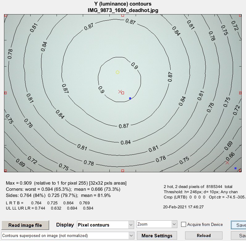
Luminance contour plotshows normalized pixel level contours for the image file luminance channel, where luminance is defined as Y = 0.30*R + 0.59*G + 0.11*B. This light falloff is sometimes called "vignetting". A maximum value of 1 corresponds to pixel level = 255 for image files with a bit depth of 8 or 65535 for a bit depth of 16. Some illumination nonuniformity is evident in the plot: the top is brighter than the bottom. The image is smoothed (lowpass filtered) before the contours are plotted. The text displays the maximum normalized pixel level for the luminance channel, the worst and mean corner values (in normalized pixel levels and as a percentage of maximum), and the side values. Selected EXIF data is shown on the right. Two hot (¤) and two dead (•) pixels (which were simulated) were detected with pixel level thresholds of 246 and 10 (of 255), respectively. Details below. Some image editors have a function that corrects vignetting (though it may be desirable to keep some vignetting for aesthetic reasons). |
 |
|
shows normalized pixel level contours for the image file luminance channel. A maximum value of 1 corresponds to pixel level = 255 for image files with a bit depth of 8 or 65535 for a bit depth of 16. Some illumination nonuniformity is evident in the plot: the top is brighter than the bottom. The image is smoothed (lowpass filtered) before the contours are plotted. The side and corner regions are shown as red rectangles. The approximate location of the maximum luminance is indicated by a yellow O. 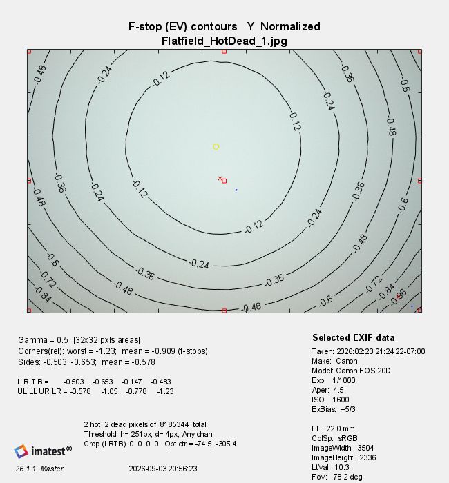 The text displays the maximum unnormalized pixel level for the luminance channel, the worst and mean corner values (in unnormalized pixel levels and as a percentage of maximum), and the side values. Selected EXIF data is shown on the right. Two hot and two dead pixels (which were simulated) were detected with thresholds of 243 and 12 (pixels), respectively. The crop (Left, Right, Top, Bottom) is shown just below. Details below.
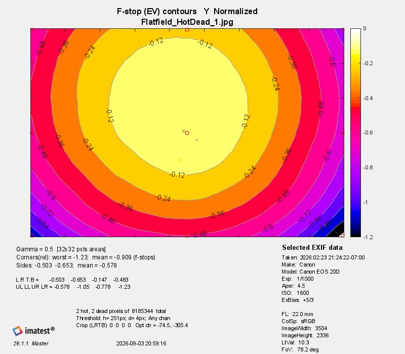
Light falloff depends on the lens aperture (f-stop) as well as a number of lens design parameters. Lenses designed designed for digital cameras, where the rays emerging from the rear of the lens remain nearly normal (perpendicular) to the sensor surface, tend to have reduced light falloff. For aesthetic purposes I generally recommend undercorrecting the image, i.e., using a larger Lens Focal Length. This makes the edges somewhat darker, which is usually pleasing. Ansel Adams routinely burned (darkened) the edges of his prints. Part of the reason was that he had to compensate for light falloff from his enlarger (when he wasn't contact printing). "My experience indicates that practically every print requires some burning of the edges, especially prints that are to be mounted on a white card, f-stop contour plotshows image file luminance contours, measured in f-stops, normalized to a maximum value of 0. A pseudocolor display with color bar has been selected. The colors in the color bar are fixed: colors always vary from white at 0 f-stops to black at -4 f-stops and darker. For this plot to be accurate, a good estimate of gamma (the camera's intrinsic contrast) is required. Gamma is measured by Color/Tone Interactive or Auto using any one of several widely-available grayscale step charts, or by legacy modules Stepchart or Colorcheck. |
F-stop contour plot in pseudocolor (normalized) |
|
It's important to measure gamma because very few cameras use the exact gamma specified by the color space. It can't be tricky to measure for several reasons. (1) (2) Many cameras have complex response curves, for example, "S"-curves superposed atop gamma curves. This means that gamma can vary with brightness. (3) Some cameras employ adaptive signal processing (local tone mapping) in their RAW conversion algorithms. This can increase local contrast, but decrease overall (large area) contrast. This can improve perceptual image quality for a wide range of scenes, but makes measurements difficult, especially since Light Falloff targets have the lowest possible contrast. Both contour plots are available as 3D plots (Master-only). The 3D plot on the right is unnormalized and shaded. |
|
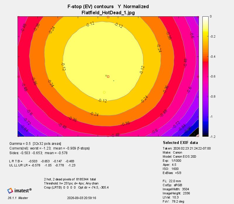
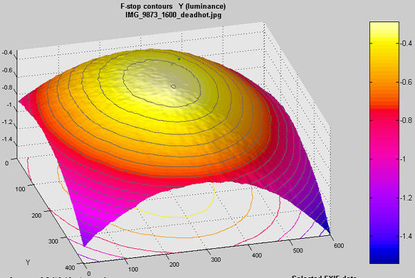 3D shaded pseudocolor F-stop contour plot (unnormalized)
The f-stop falloff in the second plot is derived from the equations,
Pixel level = k1 luminanceγ ; Luminance = k2 pixel level1/γ and
F-stop loss = log2(luminance ratio) = 3.322 log10(luminance ratio)
where luminance ratio is the ratio of the maximum luminance to the luminance in the area of interest, for example, the mean value of the corners.
Example: The first and second figures, above, are derived from the same image file. In the first figure, the mean pixel level at the corners relative to the center is 0.666/0.905 = 0.736 (73.6%). Since γ is assumed to be 0.5 (fairly typical of encoding gamma of digital cameras, the exposure at the corners relative to the center is 0.7361/γ = 0 .7362 = 0.5416. The corresponding f-stop loss = log2(0.5416) = 3.322 log10(0.5416) = -0.885 f-stops. There is a slight discrepancy with the second figure, which calculates the mean at the corners (0.894 f-stops) after taking the logarithm to convert results into f-stops.
shows image file luminance contours, measured in f-stops, normalized to a maximum value of 0. A pseudocolor display with color bar has been selected. The colors in the color bar are fixed: colors always vary from white at 0 f-stops to black at -4 f-stops and darker. For this plot to be accurate, a correct estimate of gamma (the camera's intrinsic contrast) is required. Gamma is measured by Stepchart, using any one of several widely-available step charts, or by Colorcheck.
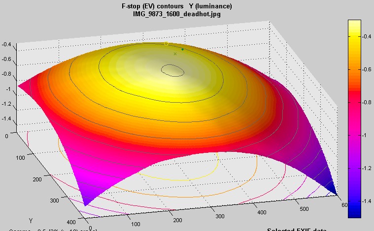
Gamma can be tricky to measure for several reasons. (1) Many cameras have complex response curves, for example, "S"-curves superposed atop gamma curves. This means that gamma can vary with brightness. (2) Some cameras employ adaptive signal processing in their RAW conversion algorithms. This increases contrast (i.e., gamma) for low contrast subjects and decreases it for contrasty subjects. This improves pictorial image quality for a wide range of scenes, but makes measurements difficult, especially since Uniformity targets have the near-zero contrast.
Both contour plots are available as 3D plots (Master-only). The following 3D plot is unnormalized and shaded. 3D plots are rarely used because they are slow (but they can be pretty).
The f-stop falloff in the second plot is derived from the equations,
Pixel level = k1 luminanceγ ; Luminance = k2 pixel level1/γ and
F-stop loss = log2(luminance ratio) = 3.322 log10(luminance ratio)
where luminance ratio is the ratio of the maximum luminance to the luminance in the area of interest, for example, the mean value of the corners.
Example: The first and second figures, above, are derived from the same image file. In the first figure, the mean pixel level at the corners relative to the center is 0.666/0.905 = 0.736 (73.6%). Since γ is assumed to be 0.5 (fairly typical of encoding gamma of digital cameras, the exposure at the corners relative to the center is 0.7361/γ = 0 .7362 = 0.5416. The corresponding f-stop loss = log2(0.5416) = 3.322 log10(0.5416) = -0.885 f-stops. There is a slight discrepancy with the second figure, which calculates the mean at the corners (0.894 f-stops) after taking the logarithm to convert results into f-stops.
Additional figures are illustrated in Flat Field Figure 2.
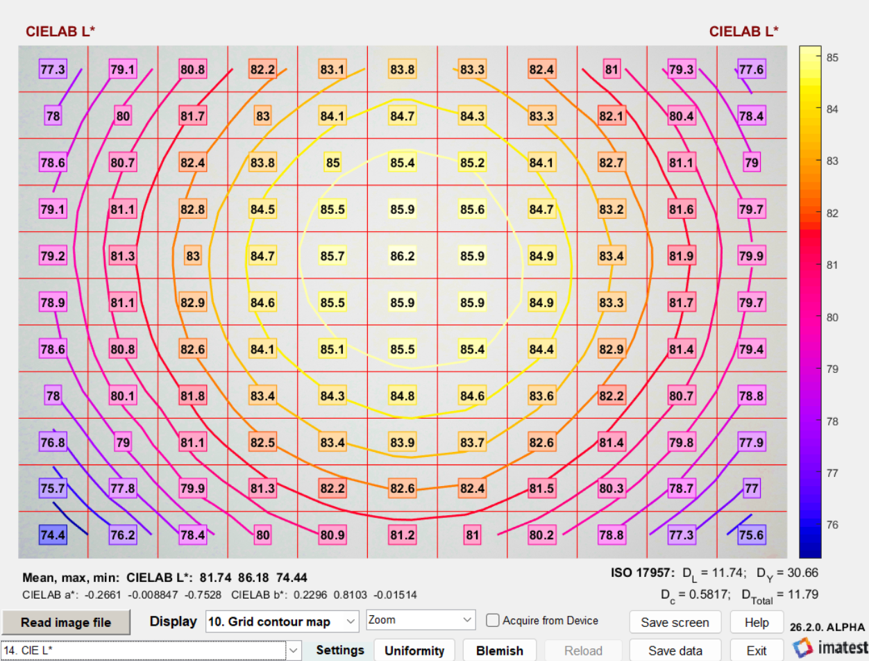
Grid contour map
The grid contour map, introduced in Imatest 2020.2, is particularly good for visualizing results. It works very well in Uniformity Interactive because you can quickly scan through different results. Unlike the grid plot, which displays two or three values in the grid (and is difficult to read), it displays only one value. But this isn't much of a drawback because it's easy to scroll through the results.
| Display 1. Mean (Y-pixel) 2. Sigma (Y-pixel) 3. S/N (Y-pixel) 4. SNR dB (Y-pixel) 5. Delta-C 6. Delta-E 7. Delta-C 94 8. Delta-E 94 9. Delta-C 00 10. Delta-E 00 11. R/B pixel ratio 12. R/G pixel ratio 13. B/G pixel ratio 14. CIE L* 15. CIE a* 16. CIE b* 17. Red 18. Green 19. Blue 20. CIE X 21. CIE Y 22. CIE Z 23. CIE x 24. CIE y |
Grid contour map for L* in Uniformity Interactive. |
Hot and dead pixels
of 8185344 total
Threshold: h= 245; d= 10
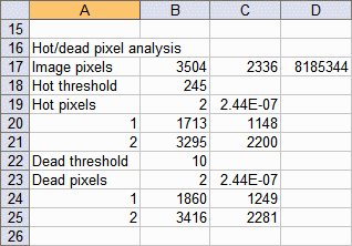
Imatest Master allows you to detect hot and dead pixels. Hot pixels are stuck at or near the sensor's maximum value (255 in 8-bit files); dead pixels are stuck at or near 0. Image processing (especially demosaicing and data compression) may alter these numbers. Thresholds lower than 255 and higher than 0 are usually required, particularly for JPEG files, where isolated pixels are smeared, even for the highest quality levels. Hot and dead pixels cannot be reliably detected in JPEGs saved at lower quality levels.
The hot and dead pixels shown on the right met the criteria that they were above or below the threshold for any color channel. All channels or the selected channel could have been selected.
The first figure in Uniformity shows two simulated hot (x) and dead (•) pixels. The CSV output file on the right shows the basic statistics for the image (8185344 pixels total). h = 245 and d = 10 are the hot and dead pixel thresholds, respectively. The number and fraction of the hot and dead pixels are shown, followed by the x and y-locations of the first 100 hot and dead pixels. The Histogram plot, described below, is useful for selecting thresholds.
Optical Center
The optical center is the approximate geometric location of the brightest part of the image. It has to be calculated very carefully using a centroid calculation (which is mathematically similar to center of gravity) because noise makes the very broad peak location unreliable— even with highly smoothed images. The horizontal (x) and vertical (y) Optical Centers are calculated separately using the same algorithm. We describe the horizontal calculation.
- Find the mean value (Lmean(x)) of a horizontal band that runs across the image and extends from 0.25 to 0.75 the image height (i.e., half the image height).
- Smooth (lowpass filter) Lmean(x).
- Find the peak value of smoothed Lmean(x). Call it LpeakX. (The peak location is not a stable indicator of the Optical Center.)
- The X-Optical Center is the centroid of the object defined by G(x) = Lmean(x) - 0.95*LpeakX where Lmean(x) > 0.95*LpeakX .
The equation is X-Optical Center = ∫x G(x) dx ⁄ ∫G(x) dx .
Optical center is displayed as a yellow circle ("O") in luminance contour plots and is reported in the CSV and JSON output files.
Note that the optical center (for illumination) described here is one of three optical centers measured by Imatest (the others are center of distortion and center of sharpness).
Color shading (nonuniformity)
The Color shading plot displays the ratio or difference between R, G, and B channels or L*a*b* color differences (ΔE, ΔC, ΔE94, ΔC94, ΔE00, or ΔC00 ). Two examples are illustrated below. The first shows shading as the ratio of Red to Blue (R/B) channel pixels. Plotted results have been normalized to a maximum of 1.0. Normalization only affects the plots; it makes the plotted results relatively insensitive to white balance errors. The background displays the image with exaggerated colors (HSV saturation S has been increased by 10x for low saturation values; less for high values.)
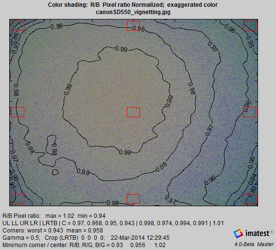
Normalization refers to the plot-only. The numbers displayed below the plot are not normalized.
The R/B Pixel ratio max and min (1.02 and 0.94, above (unnormalized)) are taken over the entire smoothed image (not restricted to the corner and side areas indicated by the red rectangles). For this reason they tend to be more extreme than the maxima and minima of the squares (displayed on the next line), and the ratio between them (0.94/1.02 = 0.92) is generally lower than the minimum ratio between the center and the sides & corners. They are calculated and included in numeric outputs (CSV, JSON, and XML files) only when the Color shading plot is produced. Other values (from fixed regions) are always calculated and included in numeric outputs. Two out of twenty-nine of these results are shown in the CSV and JSON examples below.
| Pixel ratios | R/B | R/G | R/B | B/R | G/R | B/G | ||||||||
| Maximum | 1.017 | 1.006 | 1.015 | 1.064 | 1.054 | 1.025 | ||||||||
| Minimum | 0.94 | 0.949 | 0.975 | 0.983 | 0.993 | 0.984 | ||||||||
| Detailed color shading analysis: Imatest 3.7+ | ||||||||||||||
| Result | Center | UL | LL | UR | LR | L-Ctr | R-Ctr | T-Ctr | B-Ctr | Ctr 25% | Worst corner | Mean corner | Best corner | Pct corner var |
| R/B unnorml | 1.013 | 0.97 | 0.968 | 0.95 | 0.943 | 0.998 | 0.974 | 0.994 | 0.991 | 1.012 | 0.943 | 0.958 | 0.97 | 2.828 |
| R/G unnorml | 1.005 | 0.98 | 0.979 | 0.961 | 0.963 | 0.994 | 0.984 | 0.997 | 0.994 | 1.004 | 0.961 | 0.97 | 0.98 | 1.945 |
| B/G unnorml | 0.991 | 1.009 | 1.01 | 1.011 | 1.021 | 0.996 | 1.01 | 1.003 | 1.003 | 0.992 | 1.009 | 1.013 | 1.021 | 1.122 |
JSON output. Values in the image are highlighted.
"pixel_color_stats": "Pixel ratios, R/B, R/G, R/B, B/R, G/R, B/G,",
"maximum_stat": [1.017,1.006,1.015,1.064,1.054,1.025],
"minimum_stat": [0.9396,0.9487,0.975,0.9829,0.9933,0.9844],
"resTable_comment": "Results table variables start with resTable_.",
"resTable_entries": "Center, UL, LL, UR, LR, L-Ctr, R-Ctr, T-Ctr, B-Ctr, Center 25%,Worst corner, Mean corner, Best corner, Pct corner var",
"resTable_R_div_B_unnorml": [1.0134,0.9702,0.96837,0.95031,0.94276,0.99793,0.97397,0.99369,0.99091,1.0124,0.94276,0.95791,0.9702,2.828],
"resTable_R_div_G_unnorml": [1.0047,0.97956,0.97873,0.9605,0.96265,0.99398,0.98409,0.99673,0.99411,1.0043,0.9605,0.97036,0.97956,1.945],
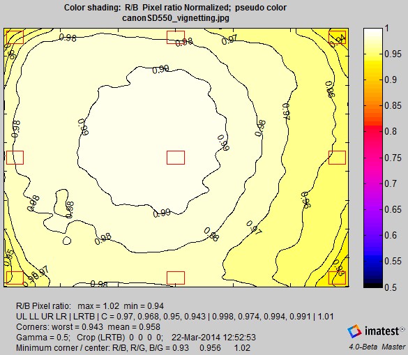
The second example shows the R/B ratio in pseudocolor. (The difference in f-stops could also be displayed, but is not shown here.) Plotted results have been normalized to 1.0.
Color nonuniformity can be displayed as one of the L*a*b* color difference metrics (ΔE = sqrt(ΔL*2 + Δa*2 + Δb*2 ), ΔC = sqrt(Δa*2 + Δb*2 ), ΔE94, ΔC94, ΔE00, ΔC00 ), referred to the center of the image (either the central region, with size specified in the Corner and side regions box or the central 25% by area). The ΔC metrics are of particular interest for color metrics because they omit luminance differences (ΔL*). It is displayed below as a 3D plot, which can be rotated for enhanced visualization..
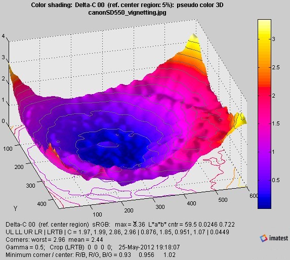
The Extra smoothing box should always be checked for 3D plots.
Uniformity profiles
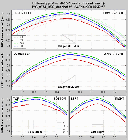
Uniformity profiles displays profiles of image levels along several lines: Diagonal Upper Left-Lower Right, Diagonal Lower Left-Upper Right, Vertical Top-Bottom (center), and Horizontal Left-Right (center). Several display options are listed below.
| RGBY unnormalized (max 1) |
| RGBY unnormalized pixels (max 255) |
| RGBY normalized (max 1) |
| Ratios: R/G, B/G (G constant) |
| RGBY normalized: ALL CHANNELS |
| Delta L* a* b* C* (C* = chroma) |
The independent axis goes from 0 to 1 in steps of 0.025 (41 steps total). Detailed results for the 41 steps are written to the CSV and XML output files.
Polynomial fit A fourth order fit to R, G, and B (or L*, a* and b*) is shown as faint dotted lines in the upper (Diagonal UL-LR) plot. The equation for the fit is
y = c1r4 + c2r3 + c3r2 + c4r + c5
where r is the distance from the center normalized to the center-to-corner distance (r = 1 at the corners). The Y-fit line is calculated from the R, G, and B fit lines using luminance coefficients, and thus does not have separate polynomial fit coefficients. The R, G, and B coefficients are in displayed the CSV and JSON output files. They have the following format in the CSV output file:
|
Fourth order fit: y = c(1)*r^4 + C(2)*r^3 + ... + c(5) where r is normalized to center-to-corner. | |||||
| R | 0.045 | -0.108 | -0.081 | -0.083 | 0.866 |
| G | -0.124 | 0.207 | -0.295 | -0.037 | 0.922 |
| B | -0.189 | 0.315 | -0.341 | -0.037 | 0.907 |
Grid plot
Several grid choices (3x3 through 32x18) and plot calculations are available.
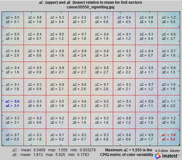
For the grid plot, which implements the CPIQ Phase 2 specification, the mean of the entire image is used as the reference for calculating ΔC and ΔE.
Histograms
The histogram plot, introduced in Imatest Master 2.3.11 (July 2007), facilitates the detection and the setting of thresholds for stuck (hot, dead, etc.) pixels. Histograms of log10(occurrences+1) are displayed for the red, green, and blue channels. [The logarithm compresses the plot so even a single bad pixel is visible. log10(occurrences+1) is used because log(0) = −∞ (minus infinity), while log(1) = 0.]
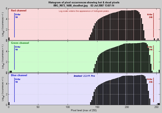
In this example, single stuck pixels are plainly visible near levels 0 and 252. Although these stuck pixels were synthesized, their levels is slightly different due to JPEG compression (they were the same in a TIFF file). The dead pixel threshold is shown on the left in blue; the hot pixel threshold is shown on the right in red. You can quickly see if the thresholds are set correctly— if they are outside the valid density region and if the dead and hot pixels are above and below their respective thresholds. You can change threshold settings and rerun Uniformity if necessary.
Noise detail
shows an exaggerated or pseudocolor image of the noise detail with long-range density variations removed. Four options are available:
| Exaggerated local noise (standard) | Exaggerated image of local noise |
| Local noise with added contours | Exaggerated image of local noise with added contours |
| Pseudocolor contours with colorbar | Pseudocolor image of local density variations. The image has been smoothed. Colors vary from image to image: the color map covers the density range of the image. |
| Spot detection w / threshold (pseudocolor) | Pseudocolor image emphasizing spots. Fixed color map. Image is normalized to the mean density. For clarity, only densities between 0.9 and 1 are displayed in the color map. |
| 3D Pseudocolor Contours shaded | 3D pseudocolor image may be rotated for enhanced visualization. Shading emphasizes contour shapes. |
| 3D Pseudocolor Contours | The Colormap (which relates color to levels) is more accurate without shading. |
| 3D Inverted Pseudocolor Contours shaded | Inverts the data (Z-axis) |
| 3D Inverted Pseudocolor Contours | |
| 3D Spot detection, pseudocolor shaded | 3D spot detection. The Z-axis is always inverted so spots stand out. |
| 3D Spot detection, pseudocolor |
The local noise figures are produced by
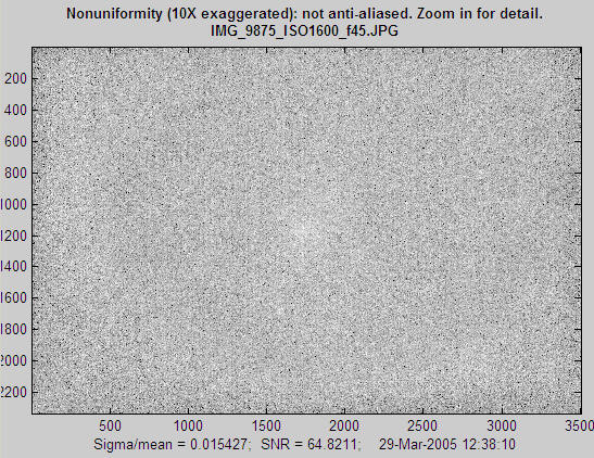
- Subtracting a highly smoothed version of the image from the image itself. This removes broad image variations (low spatial frequencies), leaving only the fine detail. (The signal is highpass filtered.) Exaggerating the fine detail by a factor 5x or 10x, depending on the signal-to-noise ratio (the average pixel level of the original image divided by the standard deviation of the difference image (the results of step 1), i.e., the RMS noise). Adding an offset to the the exaggerated signal so the average level of the image is displayed as middle gray.
- If Local noise with added contours is selected, contours are calculated by subtracting the same highly smoothed version of the image from a moderately smoothed version of the image. Smoothing is necessarily because noise would make the contours unintelligibly rough.
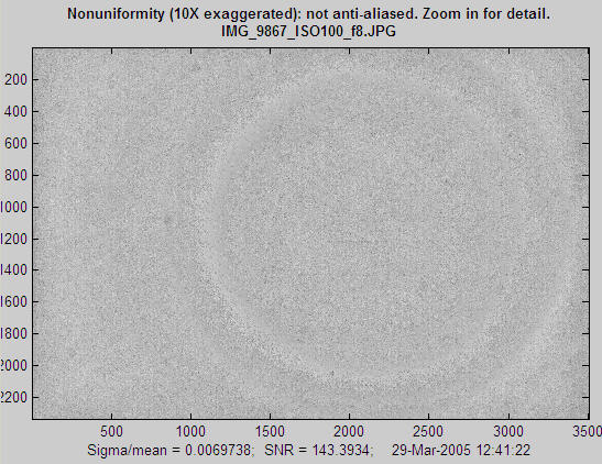
The first image (below) shows noise detail for the Canon EOS-20D at ISO 1600 with the 10-22mm lens set to f/4.5. No surprises here; electronic noise dominates.
The second image (below) shows noise detail for the Canon EOS-20D at ISO 100 with the 10-22mm lens set to f/8. Thanks to the small aperture, some very faint dust spots are visible. The dust is on the anti-aliasing/infrared filter/microlens assembly in front of the sensor. This assembly can be well over 1 millimeter thick. Stopping the lens down (increasing the f-stop setting) reduces the size of dust spots but makes them darker. This image has a surprise in the form of concentric circles: bands where the noise appears to be higher or lower than the remainder of the image. This may be caused by (a) the Analog-to-Digital (A-D) converter in the image sensor chip, which can have small discontinuities when, for example going from level 127 to 128: binary 01111111 to 10000000, or (b) JPEG artifacts. Rrecall that these noniniformities are exaggerated by a factor of 10: they would be invisible or barely visible on an actual image; you might seem then faintly in smooth areas like skies.
Here is the same image, displayed in pseudocolor (which shows the amount of variation) with a color bar, and including a histogram (of individual pixels, not the smoothed image used to generate the contour plot on the left). The scale varies from image to image; it is not fixed like the scales for for the luminance and f-stop contour plots (which display long range, low spatial frequency variations). The histogram is narrower than the separate histogram image (above) because long-range (low spatial frequency) density variations have been removed. It is a good approximation to the average sensor noise. The circular pattern may originate with reflections between the light source, lens, and sensor.
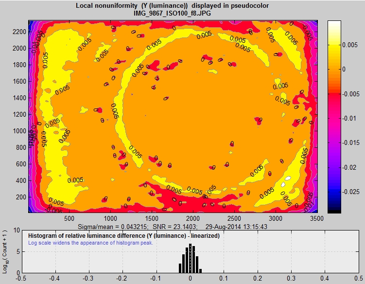 Local nonuniformities shown in pseudocolor, Canon EOS-20D, ISO 100, 10-22mm lens, f/8.
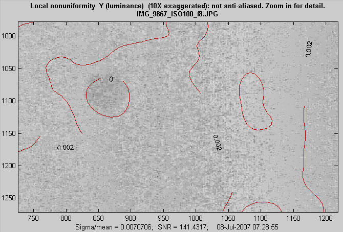
The image below is an enlargement (a zoom) of the above image, centered on the dust spot to the left of the center. You can zoom into an image by using the mouse to draw an rectangle, or by simply clicking on a feature you want to enlarge. You can restore the original image by double-clicking anywhere on the image.
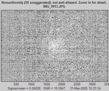
The following image is the noise detail from a 2 f-stop underexposed image with maximum luminance = 0.161 (out of 1), f/4.5, ISO 100. It shows a clear pattern. Although it looks alarming, this pattern is invisible because (a) it is in a very dark region, (b) it is aliased. The actual pattern has a much higher spatial frequency, hence is less visible. You need to zoom in to view the true pattern, which is less visible than it appears here.
Spot detection (better with Blemish Detect)
| Note: Spot detection is handled with much more detail and greater accuracy in Blemish Detect, which allows blemish filtering and thresholds to be tuned so that visible blemishes are flagged and invisible blemishes (below the visible threshold) are ignored. The filtering is based on an understanding of the human eye. |
Because Spot detection works so much better in Blemish Detect, the description will be hidden unless you press the button below.
Show moreShow less
When Spot detection w / threshold (pseudocolor) is selected in the Noise detail popup menu, the pseudocolor display emphasizes dark spots (the type that result from dust on the sensor) and minimizes noise, light spots, and long range density variations. The following webcam image (originally 1600 pixels wide) has two rows of five simulated spots (added by an image editor). Other irregularities are from the sensor itself.
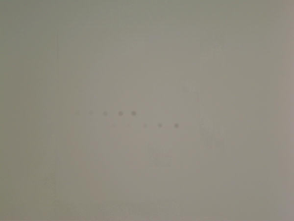
Webcam image with 10 simulated spots (5 in each of 2 rows)
With the standard Pseudocolor contours with colorbar display, the darker spots are clearly visible, but the lighter spots are lost in the overall density variations.
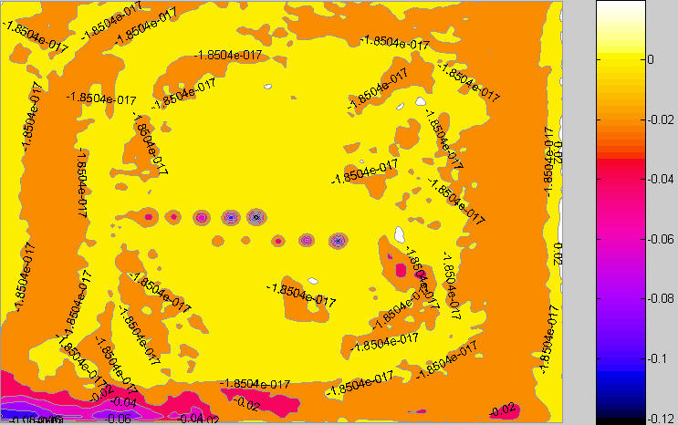
Image with spots: standard pseudocolor display
But they stand out in the Spot detection display. The differences in the algorithms are described below.
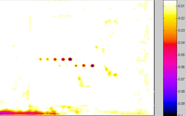
Image with spots: Spot detection display
When Pseudocolor contours with colorbar is selected, the image is normalized to its average level. Then the local variations are calculated by subtracting a highly smoothed version of the image from a moderately smoothed version of the image. This is the same data used for the contours in the Local noise with added contours display, described above. When Spot detection w / threshold (pseudocolor) is selected, there are several differences.
- The "highly" smoothed version of the image is less aggressively smoothed. This emphasizes local variations more strongly.
- The contour plot has a fixed color map, showing only values between = -0.005 (-0.5%), which is about the threshold of visibility for a spot, and -0.1 (-10%), which is the density for a highly visible spot. All values above -0.005 are displayed as white and all values below -0.1 are displayed as black. The color map for the standard pseudocolor plot is variable, based on the minimum and maximum values of the processed image.
This approach removes much of the interfering detail from the final plot so that spots are clearly visible.

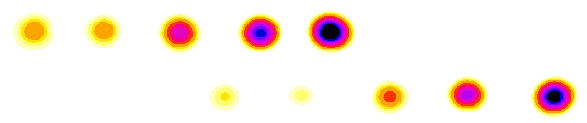
Detail: Simulated spots and Spot detection display
CSV and JSON output files
The CSV and JSON output files contain a summary of results. Most have obvious meanings.
- Image pixels contains the width, height, and total size in pixels. Hot and Dead pixels show the total count and the fraction (divided to total pixels)
- The x and y coordinates of the hot and dead pixels are listed. The maximum is 100. Coordinates are in pixels from the top-left.
They also contain EXIF data, which is image metadata that contains important camera, lens, and exposure settings. To read detailed EXIF data from all image file formats, we recommend downloading, installing, and selecting Phil Harvey's ExifTool, as described here.
Contact Imatest if you need additional .CSV output. JSON output files contain results similar to the CSV files, but can be read into external programs with a single line of code. Contents are largely self-explanatory. Contact us if you have questions or suggestions.
The .CSV output file contains additional statistics. Most have obvious meanings.
- Image pixels contains the width, height, and total size in pixels. Hot and Dead pixels show the total count and the fraction (divided to total pixels)
- The x and y coordinates of the hot and dead pixels are listed. The maximum is 100. Coordinates are in pixels from the top-left.
Contact Imatest if you need additional CSV or JSON output. The JSON output file contains results similar to the .CSV file. Its contents are also largely self-explanatory. It is stored in [root name].json.